Voltage-Gated Channels
Voltage-clamp recording
A voltage-clamp amplifier is an electronic device that uses an amplifier with feedback control to set the membrane potential to a value defined by the experimenter. The voltage-clamp amplifier maintains the membrane potential constant at that value by passing current into or out of the cell through an intracellular electrode. The membrane voltage can then be stepped to a new level and the response of the voltage-gated channels can be determined by measuring the current required to maintain that new potential. This device makes it possible to study the function of voltage-gated channels in considerable detail
Using voltage-clamp it is possible to record the sodium and potassium currents (\(I_{K}\) and \(I_{\mathit{Na}}\)) that flow through voltage-gated sodium and potassium channels during a step change in the membrane potential (Figure 1).
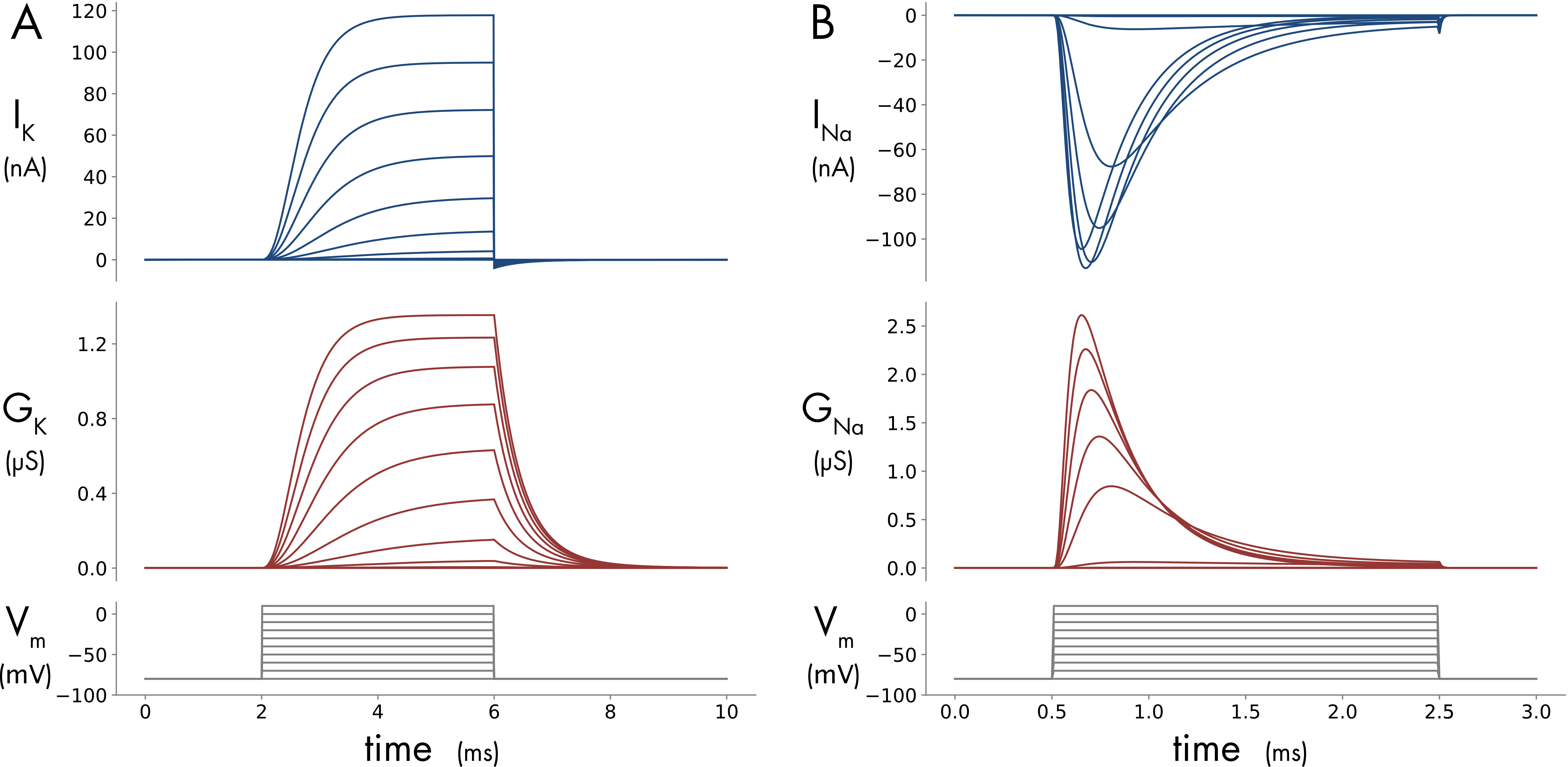
Figure 1 Simulated voltage-clamp recording in a 40 μm diameter spherical cell with voltage-gated potassium and sodium channels in the cell membrane. A. Potassium current and conductance. B. Sodium current and conductance. The voltage clamp protocol is shown in the bottom panels. Ten depolarizing steps from a holding potential of -80 mV, increasing in 10 mV increments, were applied. Note the shorter time course of the voltage steps for the sodium current. The cell membrane has a maximum specific potassium conductance of 360 pS/μm2 and a specific voltage-gated sodium conductance of 1200 pS/μm2. The Jupyter Notebook used to create this figure is provided at the bottom of this page.
Hodgkin and Huxley model of voltage-gated sodium and potassium channels
The time and voltage dependent changes of the voltage-gated sodium and potassium conductances (\(G_{K}\) and \(G_{\mathit{Na}}\)), which are proportional to the number of open channels, can then be calculated using Ohm’s law (Equations 1 and 2).
Hodgkin and Huxley interpreted their voltage-clamp results in terms of the equivalent circuit shown in Figure 2. The key change in this circuit compared to the equivalent circuit described previously is the addition of two variable conductances \({(G}_{K}\) and \(G_{\mathit{Na}})\) whose values are time and membrane voltage dependent. These conductances model the voltage-gated sodium and potassium channels in the cell membrane.
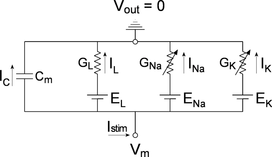
Figure 2 Equivalent circuit of an excitable cell. The arrows though the GNa and GK resistors indicate that these are variable conductances, varying with both voltage and time.
They assumed that current flow through the voltage-gated sodium and potassium channels obeyed Ohm’s law,
\[ G_{K} = I_{K}/(V - E_{K})\tag{1} \]
\[ G_{\mathit{Na}} = I_{\mathit{Na}}/(V - E_{\mathit{Na}})\ \tag{2} \]
With this assumption the voltage and time dependence of the two variable conductances \({(G}_{K}\) and \(G_{\mathit{Na}})\) could then be determined directly from the currents \({(I}_{K}\) and \(I_{\mathit{Na}})\) recorded using voltage-clamp (Figure 1). The changes in the sodium and potassium conductances reflect the summed behavior of the individual voltage gated ion channels in the membrane.
Gating probabilities and voltage-dependent rate equations
Hodgkin and Huxley devised a mathematical model to describe the voltage and time dependent behavior of the variable conductances (\(G_{K}\) and \(G_{\mathit{Na}}\)). This model has proven surprisingly resilient, especially given how little was known about the function of the channel proteins at the time. The underlying idea was that there were gating particles in the membrane, the movement of which opened or closed gates that controlled ion flow through the channel.
The model builds from the simple kinetic scheme shown in Figure 3. In the model 1-n and n are dimensionless probabilities that describe the probability of a hypothetical gating particle being in either the closed (1-n) or open (n) states.

Figure 3 Kinetic scheme for a channel gating particle with voltage dependent rates α(V) and β(V).
A key innovation was the use of voltage dependent rate constants to describe the transition between these two states. The behavior of this model is described by the following differential equation,
\[ \frac{\text{dn}}{\text{dt}} = \alpha(V)\left( 1 - n \right) - \beta(V)n\ \tag{3} \]
If it is assumed that the voltage \((V)\) remains constant, equation 3 has the following exact solution,
\[n\left( t \right) = \ n_{0} + \left( n_{\infty} - n_{0} \right)(1 - e^{- t/\tau}\ )\]
where \(\tau = 1/(\alpha + \beta)\) and \(n_{\infty} = \alpha/(\alpha + \beta)\) for a given fixed voltage and \(n = n_{0}\) when \(t = 0\).
For a continuously changing voltage, which is required to simulate the action potential, equation 3 can only be solved using numerical methods. While any of the numerical methods described in Appendix 1: Numerical Methods can be used to solve this equation the use of an implicit method has advantages that become apparent in the later sections of this chapter when simulating action potential generation in the axon. The implicit trapezoid method is an implicit second order method.
\[ n_{j + 1} = n_{j} + \frac{\mathrm{\Delta}t}{2}\left( f\left( t_{j},\ y_{j} \right) + \ f\left( t_{j + 1},y_{j + 1} \right) \right)\ \tag{4} \]
Substituting equation 3 into 4 and rearranging gives an explicit solution for time dependent changes in the gating particle n.
\[n_{j + 1} = \frac{(1/\mathrm{\Delta}t - (\alpha(V) + \beta(V))/2)n_{j} + \alpha\left( V \right)}{1/\mathrm{\Delta}t\ + \left( \alpha\left( V \right) + \beta\left( V \right) \right)/2}\]
This was the numerical method used to create Figure 1.
Potassium conductance rate equations
The next step in model construction was to fit this mathematical description of channel gating to the experimental data to describe how conductance changes with voltage (Figure 1). The time dependent behavior of the simple kinetic model (Equation 3) in response to a voltage step is shown in Figure 4A.
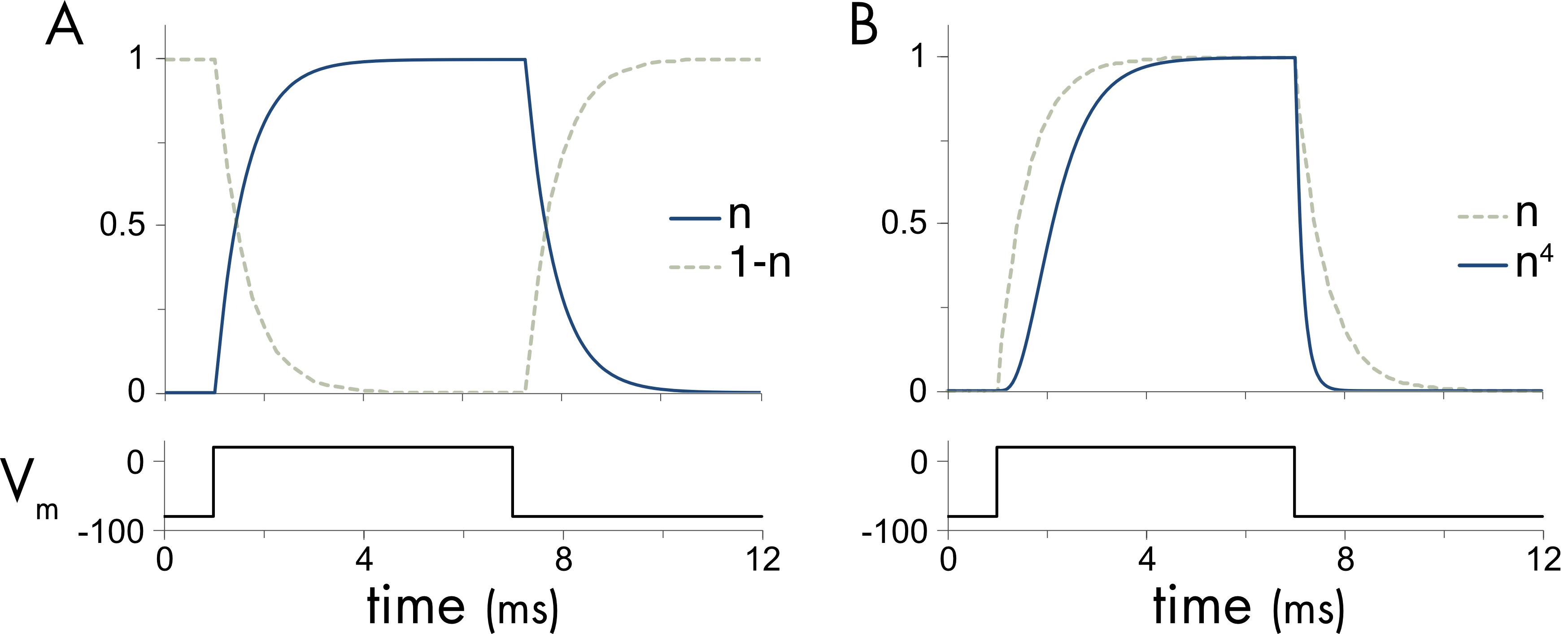
Figure 4 A. Behavior of the kinetic model shown in Figure 3 and described by equation 3, assuming that at time zero all the particles are in the closed (1-n) state and following a step change in voltage they all transition to the open (n) state at infinite time. B. For the potassium channel the n probability was raised to the fourth power to mimic the sigmoidal activation of the channel.
Immediately following a voltage step the probability the gate is in the open state \((n)\) increases from a low resting value towards the steady state value (Figure 4A). The shape of this transition following the onset of the voltage step does not perfectly match the activation of \(G_{K}\) (Figure 1), which activates sigmoidally (meaning S-shaped, most easily seen for smaller voltage steps in Figure 1). To better match the behavior of the potassium conductance the activation probability term \(n\) was raised to the fourth power. The probability \(n^{4}\) gives a closer approximation to the shape of the potassium conductance change (Figure 4B). This gating probability was incorporated into a description of potassium current flow as follows,
\[ I_{K} = G_{K}n^{4}(V - E_{K})\tag{5} \]
where, \(G_{K}\) is the total voltage-gated potassium conductance (the conductance if all the channels in the membrane were open), which is then scaled by the activation probability \(n^{4}\).
The \(n^{4}\) term describes the fraction of voltage-gated channels in the membrane that are open at a given time and voltage. It can be thought of as the probability that a given single channel will be open at that time and voltage. At resting membrane potentials this probability is low and \(n^{4}\) is close to zero. Following a voltage step to a very depolarized potential this probability increases towards a relatively high value as most of the channels open.
The final step in modeling the voltage-dependent channels required a mathematical description of the voltage-dependent rates (\(\alpha_{n}\) and \(\beta_{n}\)), which determine the rate of transition between the open and closed states. These rates were determined experimentally from voltage-clamp recordings and equations were then developed to describe the experimental data. In the Hodgkin and Huxley model the potassium channel activation rate is given by,
\[\alpha_{n}(V) = 0.01(V + 55)/(1 - \exp( - (V + 55)/10))\]
and the deactivation rate by,
\[\beta_{n}(V) = 0.125\ \exp( - (V + 65)/80)\]
These equations are plotted over a typical range of membrane potentials in Figure 5.
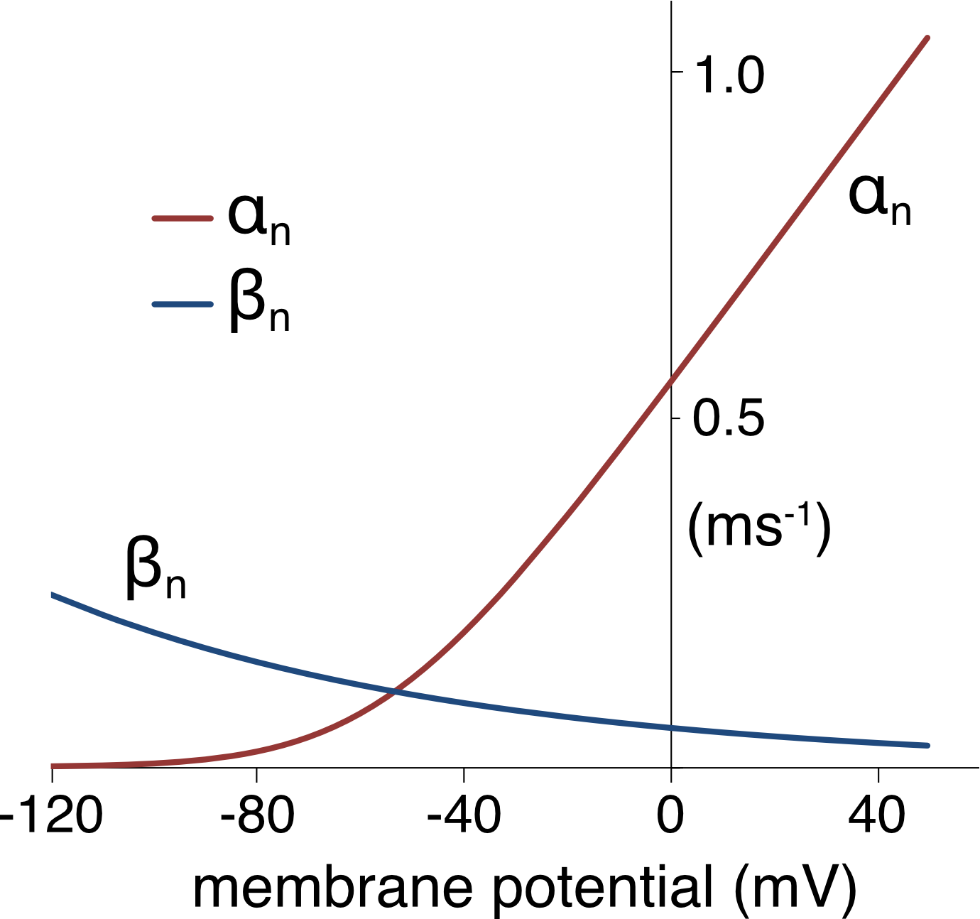
Figure 5 Voltage dependent activation α(V) and deactivation rates β(V) for the gating particle (n) of the potassium channel. Units for the y-axis scale are ms-1. The rate constants are temperature dependent and were calculated for T = 6°C.
As the membrane is depolarized the forward rate (activation rate \(\alpha_{n}\)) increases and backward rate (deactivation rate \(\beta_{n}\)) decreases. As a consequence, the probability of the channels being in the open state increases steeply with membrane depolarization.
Sodium conductance rate equations
For the sodium channel the activation particle was called m. The sodium current also activated with a sigmoidal time course and to model this behavior the activation probability was raised to the third power, \(m^{3}\). The sodium channel also inactivates. Inactivation had an approximately exponential time course. This was modeled using a single inactivation particle, h.
These gating probabilities were incorporated into a description of sodium current flow as follows,
\[I_{\mathit{Na}} = G_{\mathit{Na}}m^{3}h(V - E_{\mathit{Na}})\]
where \(G_{\mathit{Na}}\) is the total sodium conductance that is then scaled by the activation and inactivation probabilities \(m^{3}\) and h, respectively.
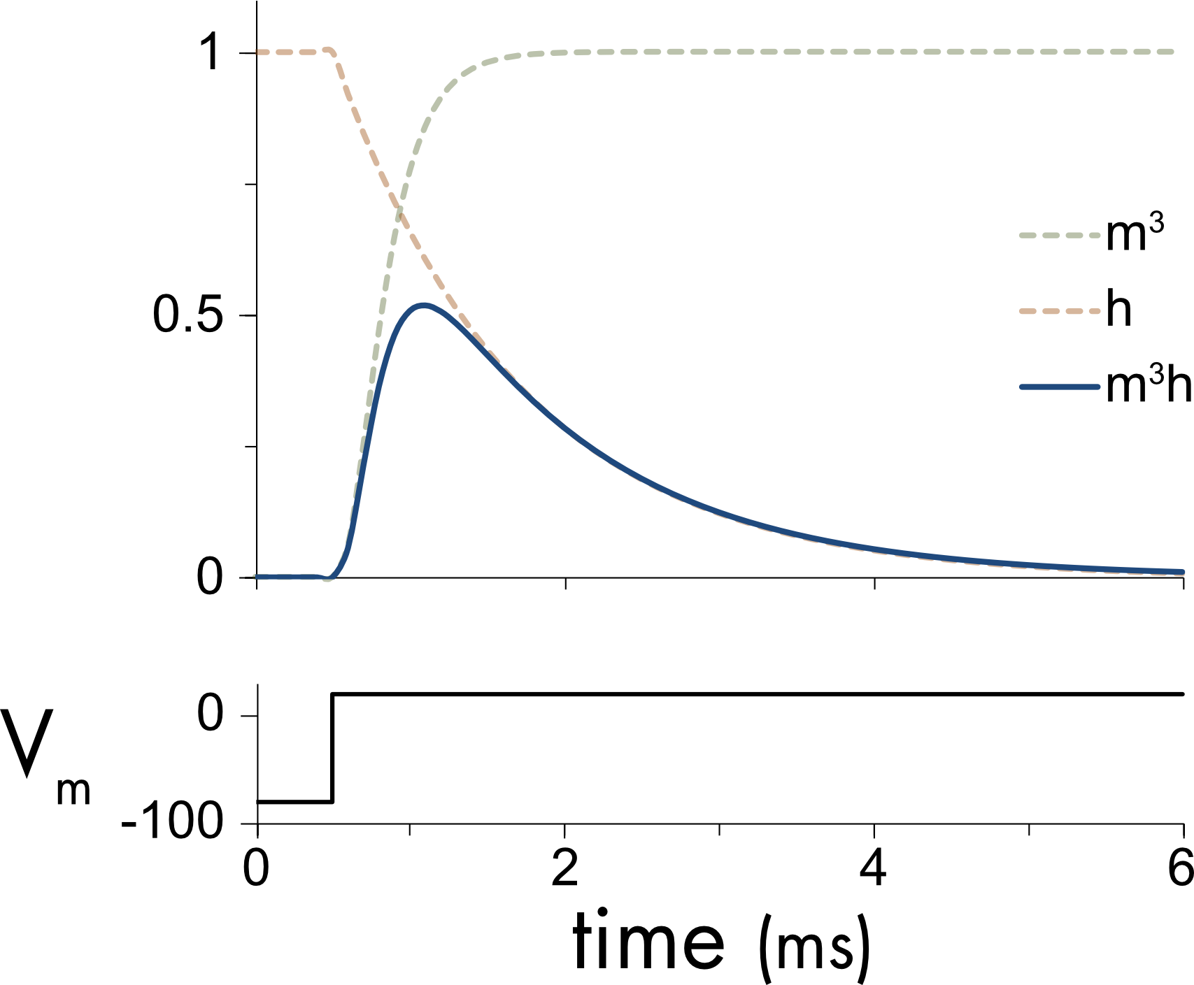
Figure 6 For the sodium channel there are two types of gating particles, to take account of the fact that the channel both activates and inactivates. The sodium activation particle, m, was raised to the third power, m3, to model the sigmoidal activation of the channel. The inactivation particle, h, controls the rate of inactivation. The voltage dependency of this particle was opposite to that of the activation particle. The sodium conductance probability is the product of these two probabilities, m3h.
The equations describing the voltage-dependent rates and their parameter values were determined empirically. The activation rate is given by,
\[\alpha_{m}(V) = 0.1(V + 40)/(1 - exp( - (V + 40)/10)\]
and the deactivation rate by,
\[\beta_{m}(V) = 4\ exp( - (V + 65)/18)\]
For inactivation, the recovery from inactivation rate is given by,
\[\alpha_{h}(V) = 0.07\ exp( - (V + 65)/20)\]
and the inactivation rate by,
\[\beta_{h}(V) = 1.0\ /\ (1 + \ exp( - (V + 35)/10))\]
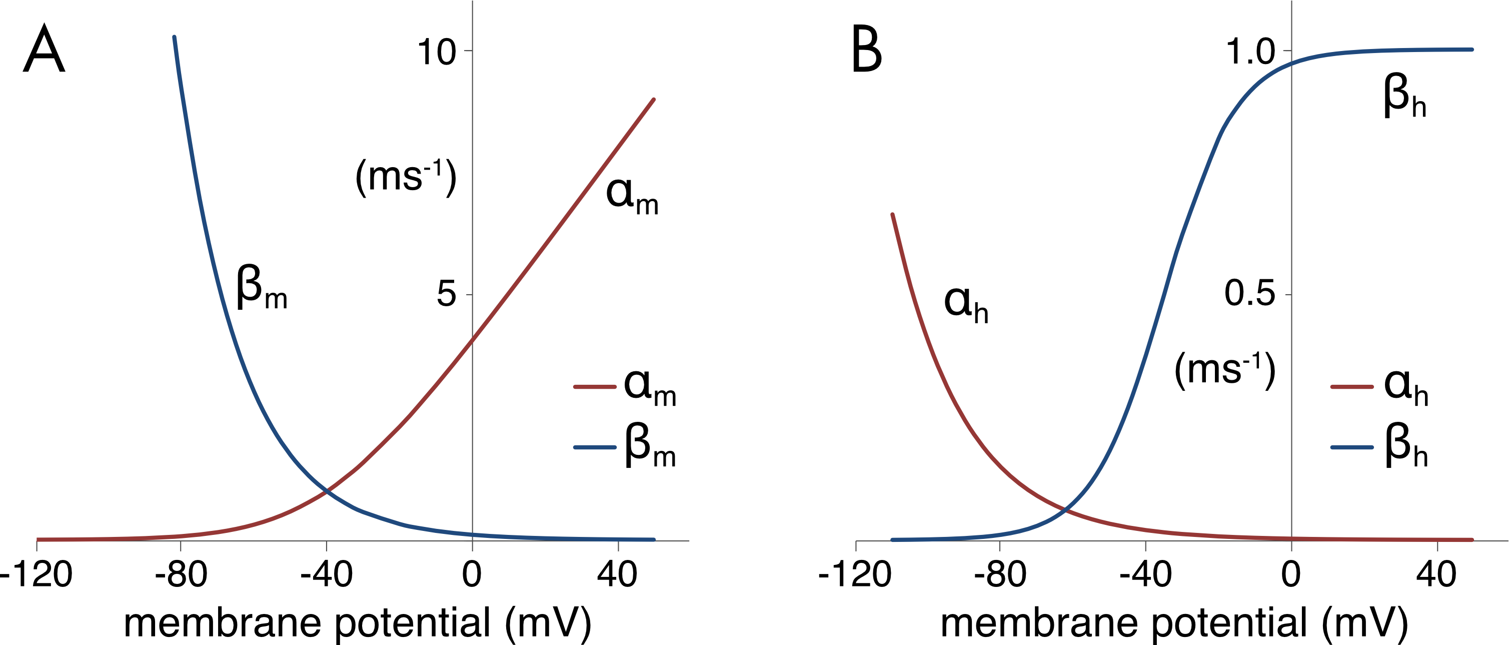
Figure 7 A. Sodium channel voltage-dependent activation and deactivation rates. B. Sodium channel recovery from inactivation and inactivation rates. The y-axis scale is ms-1. The rate constants are temperature dependent and are calculated for T = 6°C.
The activation rates (\(\alpha_{n}\) and \(\alpha_{m}\)) for both the potassium and sodium channels become much faster as the membrane potential is depolarized (Figure 5 and Figure 7). The sodium channel activation rate (\(\alpha_{m}\)) is approximately 10 times faster than the potassium channel activation rate (\(\alpha_{n}\)), which is important for determining the sequence of activation of the two channels during the action potential. The sodium channel inactivation rate (\(\beta_{h}\)) also increases with depolarization but is approximately ten times slower than the sodium channel activation rate, allowing the channel to first activate and remain open for some time before then inactivating. The rate of recovery from inactivation of the sodium channel (\(\alpha_{h}\)) is the primary determinant of the duration of the absolute refractory period following an action potential.
Jupyter Notebooks
Right click on the link to download a JupyterLab file (select ‘Save Link As…’). The files can be run locally using JupyterLab or in the cloud using Google Colab. Upload the files into Colab by selecting ‘File>Upload notebook’.