Action Potential in a Small Cell
A model of an electrically excitable cell can be created by combining the equivalent circuit model for the passive electrical properties of a small cell with the Hodgkin and Huxley model of voltage-gated channels.
Action potentials are recorded using current clamp, which means that the sum of all the different currents that flow across the membrane will equal zero,
\[I_{\text{stim}} - I_{C} - I_{L} - I_{K} - I_{\mathit{Na}} = 0\]
where \(I_{\text{stim}}\) is the stimulus current injected into the cell to trigger an action potential.
Rearranging,
\[I_{\text{stim}} = I_{C} + I_{L} + I_{K} + I_{\mathit{Na}}\]
Incorporating equations describing each of these currents,
\[I_{\text{stim}} = A{\overline{c}}_{m}\frac{\text{dV}}{\text{dt}} + A{\overline{g}}_{L}\left( V - V_{L} \right) + A{\overline{g}}_{K}n^{4}\left( V - E_{K} \right) + A{\overline{g}}_{\mathit{Na}}m^{3}h(V - E_{\mathit{Na}})\]
where \(A\) is the area of the cell, \({\overline{c}}_{m}\) is the specific capacitance, and \({\overline{g}}_{L}\), \({\overline{g}}_{K}\), \({\overline{g}}_{\mathit{Na}}\) are the specific conductances.
Simplify by calculating the cell capacitance and conductances,
\[I_{\text{stim}} = C_{m}\frac{\text{dV}}{\text{dt}} + G_{L}\left( V - V_{L} \right) + G_{K}n^{4}\left( V - E_{K} \right) + G_{\mathit{Na}}m^{3}h(V - E_{\mathit{Na}})\]
Rearranging gives the differential equation,
\[ \frac{\text{dV}}{\text{dt}} = (I_{\text{stim}} - G_{L}(V - V_{L}) - G_{K}n^{4}\left( V - E_{K} \right) - G_{\mathit{Na}}m^{3}h(V - E_{\mathit{Na}}))/C_{m}\tag{1} \]
This equation can be solved numerically in combination with the three differential equations describing the behavior of the gating probabilities,
\[ \frac{\text{dn}}{\text{dt}} = \alpha_{n}\left( V \right)\left( 1 - n \right) - \beta_{n}\left( V \right)n\tag{2} \]
\[ \frac{\text{dm}}{\text{dt}} = \alpha_{m}\left( V \right)\left( 1 - m \right) - \beta_{m}\left( V \right)m\tag{3} \]
\[ \frac{\text{dh}}{\text{dt}} = \alpha_{h}\left( V \right)\left( 1 - h \right) - \beta_{h}\left( V \right)h\tag{4} \]
Solution of these four equations describes the trajectory of the membrane potential during an action potential.
A common method used to solve this set of four equations is to solve the three rate equations first after each time step using the implicit Trapezoid method described previously. To maintain second order accuracy, equation 1 is then solved at the midpoint of the time step \(\text{Δt}\) using the backward Euler method with a half time step, i.e. at time \(t_{j} + \Delta t/2\).
\[V_{j + 1/2} = V_{j} + \Delta t/2(I_{\text{stim}} - \ G_{L}(V_{j + 1/2} - V_{L}) - G_{K}n^{4}\left( V_{j + 1/2} - E_{K} \right) - G_{\mathit{Na}}m^{3}h(V_{j + 1/2} - E_{\mathit{Na}}))/C_{m}\]
which can be rearranged to give an explicit solution for \(V_{j + 1/2}\),
\[V_{j + 1/2} = \frac{V_{j}(2C_{m}/\Delta t) + I_{\text{stim}} + \ G_{L}V_{L} + G_{K}n^{4}E_{K} + G_{\mathit{Na}}m^{3}hE_{\mathit{Na}}}{2C_{m}/dt + G_{L} + G_{K}n^{4} + G_{\mathit{Na}}m^{3}h}\]
The voltage is then linearly advanced an additional half-step to complete the cycle for each \(\text{Δt}\).
\[V_{j + 1} = 2V_{j + 1/2} - V_{j}\]
This method is second order accurate for V. Although this system of equations is not stiff for a single compartment and can be solved using any of the methods outlined in Appendix 2, the system becomes increasingly stiff as more membrane compartments are added, as will be seen for the axon described in later sections, and this method can be shown to reliably converge under these more stringent conditions when the explicit methods will only be conditionally stable.
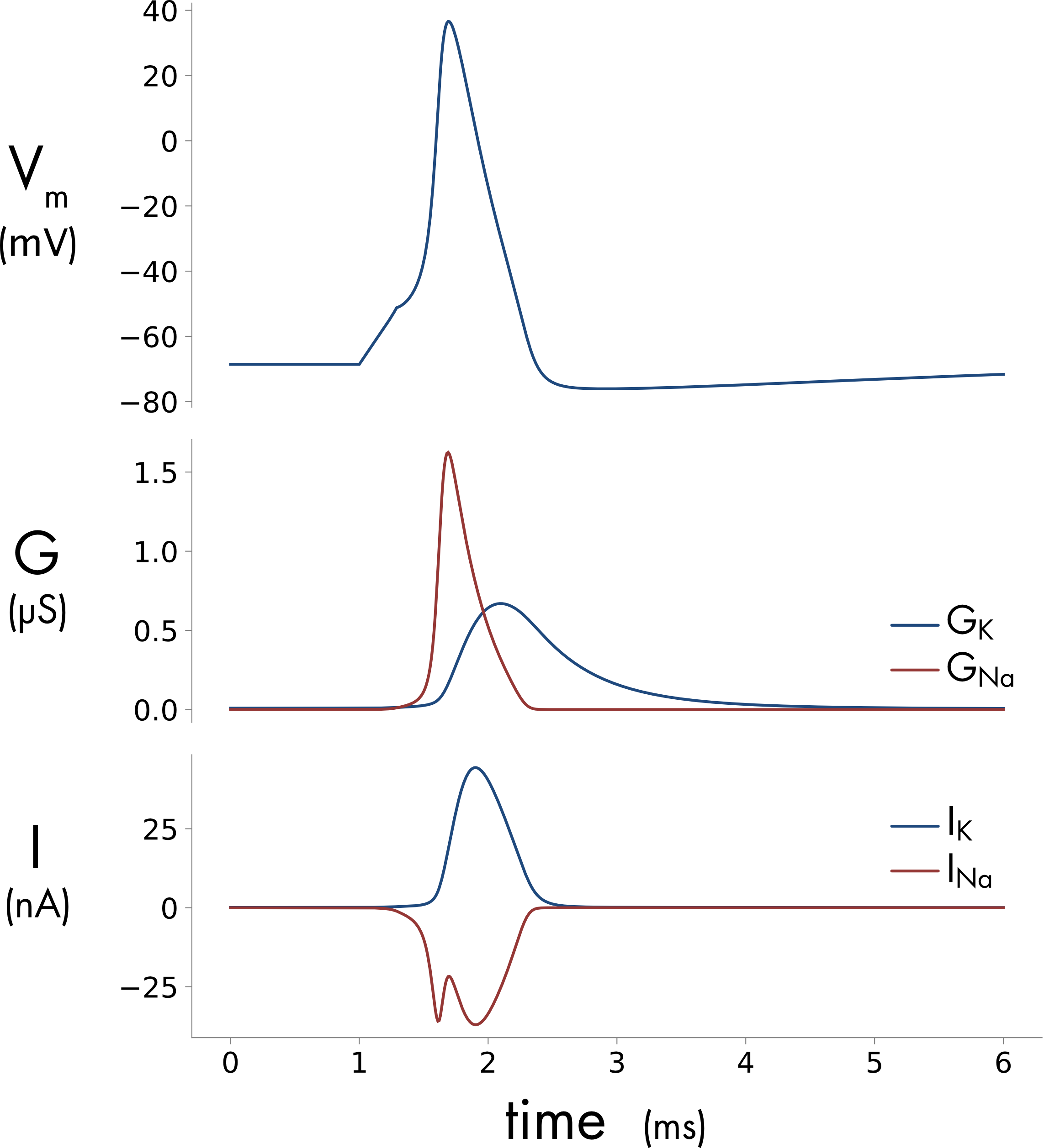
Figure 1 Simulation of an action potential in a 40 μm diameter spherical cell. A. Membrane potential B. Voltage-gated potassium (blue) and sodium (red) conductance. C. Voltage-gated potassium (blue) and sodium (red) current. The cell membrane has a specific voltage-gated sodium conductance of 1200 pS/μm2 and a specific potassium conductance of 360 pS/μm2.
Simulation of an action potential in a small cell is shown in Figure 1. The sodium conductance \((G_{\mathit{Na}})\) activates much more rapidly than the potassium conductance \((G_{K})\). This is due to the difference in the voltage-dependent rates of activation, both channels see the same changes in membrane potential but the voltage dependent rate constants controlling sodium channel activation are much faster, producing the faster activation of the sodium conductance. This is an essential feature of the system because it is the initial inrush of sodium ions that generates the rising phase of the action potential.
Jupyter Notebooks
Right click on a link to download a JupyterLab file (select ‘Save Link As…’). The files can be run locally using JupyterLab or in the cloud using Google Colab. Upload the files into Colab by selecting ‘File>Upload notebook’.