Implicit Methods

Backward Euler Method

The backward Euler method is given by the following formula

\[ y_{n + 1} = y_{n} + \mathrm{\Delta}t \cdot f\left( t_{n + 1},y_{n + 1} \right)\text{\ \ \ \ }\tag{1} \]

This has the same form as the forward Euler method, with \(f\left( t_{n + 1},y_{n + 1} \right)\) substituted for \(f\left( t_{n},y_{n} \right)\). It has a similar geometrical interpretation except that the slope is now calculated at the end of the time step rather than the beginning. For explicit methods all the terms on the right-hand side of the equation are known so that \(y_{n + 1}\) can be determined explicitly. For the backward Euler method \(y_{n + 1}\) appears on both sides of the equality, which means that some work must be invested to evaluate \(y_{n + 1}\). The amount of work required depends on the nature of the function. This is best illustrated with an example. For,

\[\frac{dy}{dt} = - y\]

using the reverse Euler method (equation 1),

\[y_{n + 1} = y_{n} + \mathrm{\Delta}t \cdot ( - y_{n + 1})\]

rearranging gives,

\[y_{n + 1} = \frac{y_{n}}{1 + \mathrm{\Delta}t}\]

In this case it is easy to isolate an explicit solution for \(y_{n + 1}\) in terms of \(y_{n}\). In most cases this is not as straightforward, and it will be necessary to use a numerical root-finding method to solve for \(y_{n + 1}\). This can add considerable computational overhead, making the method impractical. The significant advantage of using this implicit method is that it is more stable than the equivalent explicit method, as shown in Figure 1.

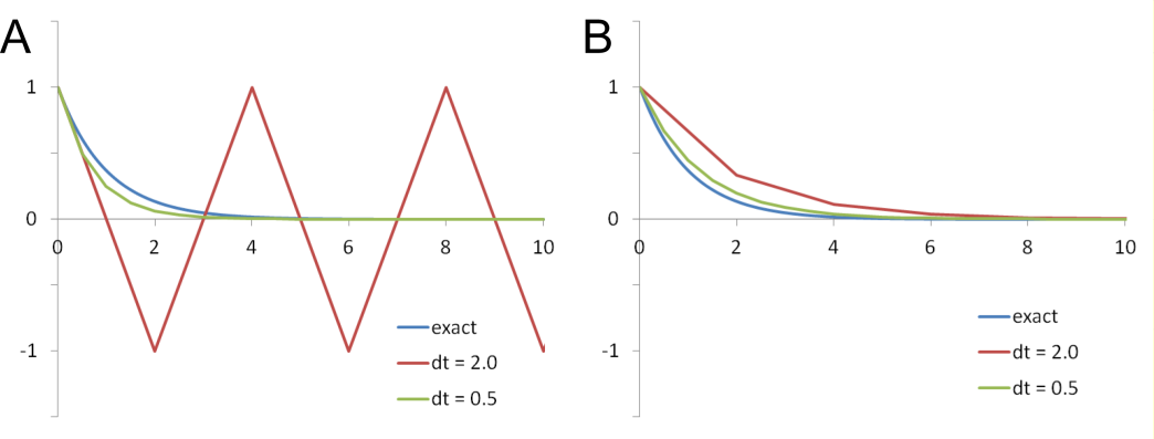
Figure 1 Comparison of forward Euler and backward Euler methods for the solution of dy/dt = -y. A. Forward Euler with exact and estimated solutions with ∆t = 0.5 and 2.0. B. Backward Euler with exact and estimated solutions with ∆t = 0.5 and 2.0. Exact solution is y(t) = e^-t.

Although the backward Euler method is 1^st order and, like the forward Euler method, is slow to converge on the exact solution with decreasing step size, it behaves much more predictably than the forward Euler at large step sizes. While the forward Euler is prone to verge into instability the forward Euler remains stable (Figure 1). This can be a significant advantage particularly when dealing with systems of differential equations in which rates of change for different variables can occur on widely varying times scales. Even if the solution for some variables is not especially accurate an implicit method will not blow up as easily as an explicit method. Systems of differential equations that are unstable when solved using explicit methods are generally known as stiff and are best solved using an implicit method, when possible.

Implicit Trapezoidal Method

The implicit trapezoidal method is also known as the Adams-Moulton One-Step method.

\[y_{n + 1} = y_{n} + \frac{\mathrm{\Delta}t}{2}\left( f\left( t_{n},y_{n} \right) + f(t_{n + 1},y_{n + 1}) \right)\]

This is an implicit second-order method, requiring two function evaluations per step. It is a numerical average of the forward and backward Euler methods. It is the implicit analog of the explicit modified Euler method. Like the backward Euler method, it can be converted to an explicit function for certain functions such as the Hodgkin and Huxley rate equations, which are typically solved using this method.