Explicit Methods

Forward Euler Method

The forward Euler method is the easiest numerical method to understand and to program. The method is inaccurate relative to more complex methods and can be unstable. These disadvantages can be minimized to some degree by using small step sizes, but more complex algorithms are usually a better choice. Nonetheless, this method can be a good first choice to get some initial feedback on a particular problem because its inherent simplicity minimizes the chance of introducing programming errors. There are several different ways to understand the forward Euler method.

The derivative is defined as,

\[\frac{\text{dy}}{dt} = \ \lim_{h \rightarrow 0}\frac{y\left( t + h) - y(t \right)}{h}\]

The discrete form of this equation is,

\[\frac{dy}{dt} \approx \frac{y\left( t + \text{Δt}) - y(t \right)}{\mathrm{\Delta}t}\]

Given,

\[\frac{dy}{dt} = f\left( t,y \right)\]

Then,

\[\frac{y_{n + 1} - y_{n}}{\mathrm{\Delta}t} = f\left( t_{n},y_{n} \right)\]

Rearranging gives the forward Euler method,

\[ y_{n + 1} = y_{n} + \mathrm{\Delta}tf\left( t_{n},y_{n} \right)\text{\ \ \ \ }\tag{1} \]

which is used to march across the interval \(0 \leq t \leq T\).

\[\begin{aligned}y_{0} &= \ y_{0}\\\\[-2ex] y_{1} &= \ y_{0} + \ \Delta tf\left( t_{0},y_{0} \right)\\\\[-2ex] y_{2} &= \ y_{1} + \ \Delta tf\left( t_{1},y_{1} \right)\\\\[-2ex] \text{...}\\\\[-2ex] y_{N} &= \ y_{N - 1} + \ \Delta tf\left( t_{N - 1},y_{N - 1} \right)\end{aligned}\]

It is an explicit method because at every step all the variables on the right-hand side of the equation are known, making computation of the next step trivial.

The geometric interpretation is illustrated in Figure 1. The differential equation \(dy/dt = f(t_{n},y_{n})\) gives the tangent or slope at any point along the curve,

\[\text{slop}{\text{e\ of\ curve\ at}\text{\ t}}_{n} = f\left( t_{n},y_{n} \right) = \frac{\text{rise}}{\text{run}} = \frac{y_{n + 1} - y_{n}}{\mathrm{\Delta}t}\]

which again gives equation 1.

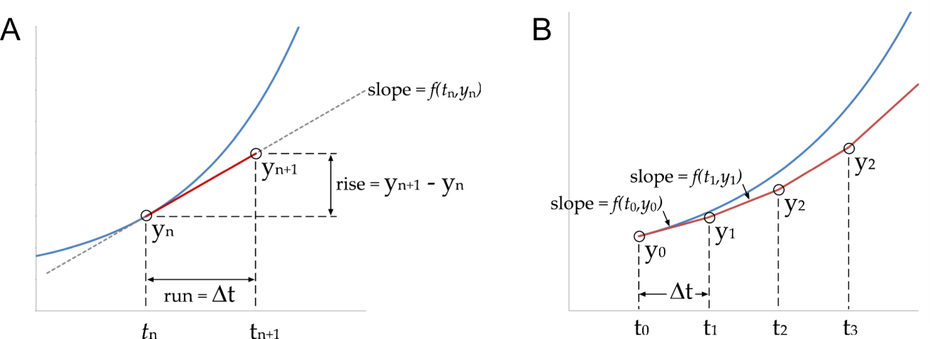
Figure 1 A) Forward Euler method. The exact solution is the blue line and the forward Euler estimate for one step\(\ \text{Δt}\) is shown in red. B) The forward Euler estimate for successive steps of \(\text{Δt}\).

To begin the march across the entire time interval the tangent at \(t_{0}\) is projected forward a distance of \(\mathrm{\Delta}t\) to \(t_{1}\) (Figure 1). It is then assumed that \(y_{1}\) is on or close to the curve at \(t_{1}\) and the tangent \(dy/dt = f(t_{1},y_{1})\) is evaluated again and the process repeated. Clearly errors in this process are unavoidable and they can accumulate.

A third way to derive the forward Euler method is from the Taylor series expansion of \(y\) about \(t\).

\[y\left( t + \mathrm{\Delta}t \right) = \ y\left( t \right) + \mathrm{\Delta}ty'\left( t \right) + \frac{1}{2}\mathrm{\Delta}t^{2}y''\left( t \right) + \frac{1}{3!}\mathrm{\Delta}t^{3}y'''\left( t \right) + \cdots\ + \ \frac{1}{n!}\Delta t^{n}y^{\left( n \right)} + \cdots\]

Truncating the Taylor series at the second term, \(\mathrm{\Delta}ty'\left( t \right)\), and rearranging for \(y'\left( t \right)\) gives,

\[y'\left( t \right)\ = \frac{y\left( t + \text{Δt} \right) - y\left( t \right)}{\mathrm{\Delta}t} + O(\Delta t)\]

where \(O(\Delta t)\) represents all the terms after the first term and is a measure of the error of the method.

Modified Euler Method

This method has multiple names, it also known as Heun’s method and the explicit trapezoidal method. The algorithm requires two evaluations of the function 𝑑𝑦/𝑑𝑡 = 𝑓(𝑡, 𝑦) for each 𝛥𝑡 step, making it twice as expensive computationally as the forward Euler method.

\[y_{n + 1}^{*} = y_{n} + \mathrm{\Delta}tf\left( t_{n},y_{n} \right)\]

\[y_{n + 1} = y_{n} + \frac{\mathrm{\Delta}t}{2}\left( f\left( t_{n},y_{n} \right) + f(t_{n + 1},y_{n + 1}^{*}) \right)\]

The first equation is simply the forward Euler method, which produces an initial prediction of \(y_{n + 1}\) called \(y_{n + 1}^{*}\). The second equation produces the corrected estimate of \(y_{n + 1}\).
This method also has a simple geometric interpretation (Figure 2). The forward Euler method is used to make an initial prediction of \(y_{n + 1}\). The slope at point (\(t_{n + 1}\), \(y_{n + 1}\)) is given by \(f(t_{n + 1},y_{n + 1}^{*})\). The corrected estimate of 𝑦 uses a numerical average of these two measures of the slope.

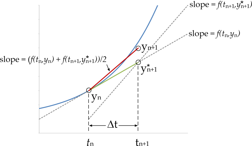
Figure 2 Modified Euler method. The exact solution (blue), forward Euler estimate (green) and modified Euler estimate (red) are shown. The modified Euler produces a notably improved estimate of \(y_{n + 1}\) compared to the forward Euler method.

Runge–Kutta Fourth Order Method

The fourth order Runge-Kutta method or RK4 requires four evaluations of the function for each time step. The marching scheme is given by the following set of equations.

\[k_{1} = \mathrm{\Delta}tf\left( t_{n},\ y_{n} \right)\]

\[k_{2} = \mathrm{\Delta}tf\left( t_{n} + \frac{1}{2}\mathrm{\Delta}t,\ y_{n} + \frac{1}{2}k_{1} \right)\]

\[k_{3} = \mathrm{\Delta}tf\left( t_{n} + \frac{1}{2}\mathrm{\Delta}t,\ y_{n} + \frac{1}{2}k_{2} \right)\]

\[k_{4} = \mathrm{\Delta}tf\left( t_{n + 1},\ y_{n} + k_{3} \right)\]

\[y_{n + 1} = y_{n} + \frac{1}{6}\left( k_{1} + \ 2k_{2} + \ 2k_{3} + \ k_{4} \right)\]

In this method \(f\left( t_{n},\ y_{n} \right)\) is the slope at the beginning of the interval [\(t_{n}\), \(t_{n} + \ \Delta t\)], \(f\left( t_{n} + \frac{1}{2}\Delta t,\ \ y_{n} + \frac{1}{2}k_{1} \right)\) is the predicted slope in the middle of the interval, \(f\left( t_{n} + \frac{1}{2}\text{Δt},\ \ y_{n} + \frac{1}{2}k_{2} \right)\) is a corrected estimate of that slope and \(f\left( t_{n + 1},\ \ y_{n} + \ k_{3} \right)\) is the slope at the end of the interval. The four estimates of the slope are averaged, giving greater weight to the two center estimates.

Accuracy of Explicit Methods

The framework for analyzing the numerical error of ODE solution methods uses the Taylor Series expansion of the solution function, \(y\).

\[y\left( t + \mathrm{\Delta}t \right) = \ y\left( t \right) + \mathrm{\Delta}ty'\left( t \right) + \frac{1}{2}\mathrm{\Delta}t^{2}y''\left( t \right) + \frac{1}{3!}\mathrm{\Delta}t^{3}y'''\left( t \right) + \cdots\ + \ \frac{1}{n!}\Delta t^{n}y^{\left( n \right)} + \cdots\]

This expansion is as a series of increasingly accurate approximations of the function \(y\). The simplest approximation to \(y\) near \(t\) is simply \(y\left( t \right)\). Addition of the second term, \(\mathrm{\Delta}ty'\left( t \right)\), forms the linear approximation to \(y\). As noted earlier this is the approximation used in the Forward Euler Method. The local truncation error of the forward Euler method is \(O(dt^{2})\) (pronounced ‘big-oh \(\text{dt}\) squared’). This is because the error term (i.e. the sum of the terms we ignored) is dominated by the term \(\frac{1}{2}\mathrm{\Delta}t^{2}\ y''(t)\). The \(dt^{2}\) term dominates because for small \(\text{dt}\), say \(dt = 10^{- 3}\), we have \(dt^{2} = 10^{- 6}\), \(dt^{3} = 10^{- 9}\), \(dt^{4} = 10^{- 12}\) and so on. Hence, the \(dt^{2}\) term is by far the largest of all the error terms.

The local accuracy of the Modified Euler Method and the Runge-Kutta 4th Order Method is determined similarly. Their local truncation errors are \(O(dt^{3})\) and \(O(dt^{5})\) respectively. This means that they match the Taylor Series expansion up to and including the \(dt^{2}\) term for the Modified Euler Method and the \(dt^{4}\) term for the RK4.

Generally, the global truncation error — the total accumulated error at the end of the simulation — is the main concern. Determination of the global truncation error relies on a theorem that roughly states, if the local truncation error is \(O(dt^{n})\) then the global truncation error is \(O(dt^{n - 1})\). This means that the Euler method is 1^st order accurate \(O(dt)\), the Explicit Trapezoid Method is 2^nd order \(O(\Delta t^{2})\)and the RK4 method is 4^th order \(O(dt^{4})\).

There are two ways to gain accuracy in solving initial value problems, decrease the step size or use a higher order and more accurate solution method. The greatest accuracy for the least amount of computational effort is desirable, where the amount of computation is determined by the number of times the function, \(f\), is evaluated. The Euler method is computationally inexpensive (only one function call per step) but has a low order of accuracy. The RK4 is more expensive (four function calls per step) but is accurate up to 4^th order.

To decide how to strike this balance use the fact that if the error of an approximation is \(O(dt^{n})\) then the error is usually roughly equal to some constant multiplied by \(dt^{n}\). For the Euler method if the step size is decreased by a factor of 4, making the computation four times as expensive, then the global truncation error also decreases by a factor of four since the global truncation error is O(dt). However, for the same computational cost we could keep the original step size but switch to the RK4 method, which would reduce the error by a factor of \(\text{dt}^{3}\). For small \(\text{dt}\) this is a much bigger improvement than we would get from decreasing the step size in the Euler method making the RK4 method a better choice.

This is shown graphically in Figure 3. The 4^th order Runge-Kutta method is remarkably accurate for large step sizes, much better than the other two methods (Figure 3A). This advantage is diminished but still retained when the comparison is controlled for equal computational effort i.e., equal number of function evaluations (Figure 3B).

 

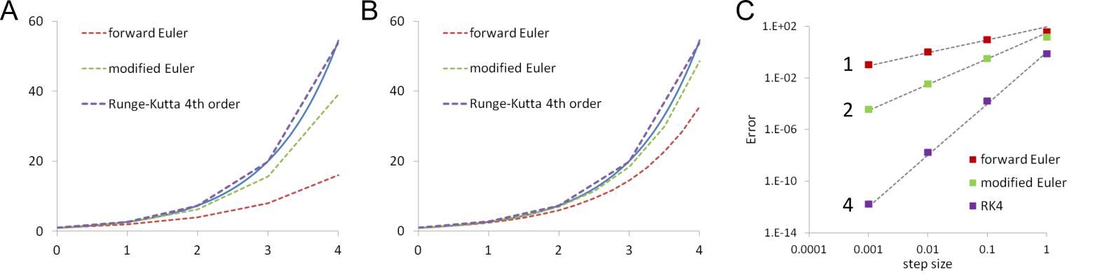
Figure 3 Comparison of forward Euler, modified Euler and Runge-Kutta 4th order methods with the exact solution of dy/dt = y. A. Equal step size. B. Equal number of function evaluations ie. the step size for the forward Euler is 4 and 2 times smaller than that for the modified Euler and Runge-Kutta method respectively. C. Effect of changing step size on error magnitude for the three methods. Dashed lines are fits to the error values with exponents of 1, 2 and 4.

The effect of the order of accuracy of a solution method can be seen using a log-log plot of the global error against the step size, \(\text{dt}\) (Figure 3C). If the method is \(O(dt^{n})\) then the errors should fall close to a straight line with gradient\(\text{\ n}\). A plot of the error versus step size for the three methods shows how much faster the error declines for the 4^th order Runge-Kutta method with decreasing step size compared to the 1^st order forward Euler method. The 4^th order Runge-Kutta produces a better estimate for less computational cost. There are diminishing returns and increased complexity with even higher order methods and the RK4 method is generally the method of choice amongst fixed step explicit numerical methods.