Passive Properties of a Small Cell
One of the earliest and most enduring successes in the mathematical modeling of biological systems has been the model devised by Alan Hodgkin and Andrew Huxley to describe the propagation of the action potential along the squid axon.1 The model is grounded in two well understood physical concepts, electric circuit theory and thermodynamics, in particular the Nernst equation. The complete mathematical description of the action potential, however, also required empirical modeling of voltage-gated channel function based on curve fitting to experimental data. These equations and the underlying model were well thought out and have become a standard method to describe the function of voltage-gated channels.
This chapter will build from the passive electrical behavior of a simple spherical cell to action potential conduction along an axon. We will start with the analysis of electrical excitation in a small isopotential cell before moving to the more complex problem of action potential propagation along a cable. The mathematical models require some understanding of differential equations, numerical methods, and linear algebra.
Equivalent Circuit of a Small Cell
The equivalent electrical circuit of a small cell is a resistor and capacitor in parallel (an RC circuit). It is assumed that the intracellular fluid is a perfect conductor and, hence, the electrical potential within the cell is the same at every point. This is known as the isopotential assumption. This assumption applies reasonably well to most small cells, irrespective of their shape, because the resistance between different regions within the cell is small relative to the resistance across the membrane. This assumption does not apply to most neurons, which have complex dendritic trees and long axons.
Another key assumption is that the lipid membrane behaves like a perfect capacitor and has essentially zero conductance for ions. For the relatively small voltages found across cells membranes this assumption holds surprisingly well.
It is also often assumed that the ion channels in the cell membrane behave as ideal resistors. For sodium and potassium channels this assumption is adequate over the voltage ranges typically studied. Over a broader voltage range the single channel conductance usually deviates from linearity in part because of the asymmetrical distribution of the ions across the membrane that support current flows — more ions can support a larger current flow. This is a particular problem for the calcium channel because of the very low internal calcium ion concentration and linearity is not generally assumed for this channel.
The equivalent circuit of a small cell is shown in Figure 1. This is known as an RC circuit, a resistor (conductor) and capacitor in parallel.
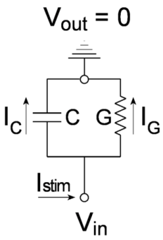
Figure 1 Equivalent circuit of a small cell. The extracellular potential is assumed to be at ground or zero potential and the internal potential (Vin) is expressed relative to this value. An injected current (Istim) has two pathways to ground, either through the membrane ion channels modeled as a resistor with conductance (G) or across the membrane capacitance (C).
Current flow across the capacitor is proportional to the rate of change of the voltage across the capacitor, where the voltage V = Vin - Vout.
\[ I_{C} = C\frac{dV}{dt}\ \ \ \ \ \tag{1} \]
Current flow through the conductance, \(G\), is given by Ohm’s Law.
\[ I_{G} = GV\ \ \tag{2} \]
A stimulus current can be applied to the center of the cell using an intracellular electrode \((I_{\text{stim}})\). From Kirchhoff’s current law, the sum of inward and outward currents at a given node in the circuit should equal zero. At the internal node, with the direction of current flow defined by the arrows in Figure 1 Kirchhoff’s law gives.
\[ I_{\text{stim}} - \ I_{C} - \ I_{G} = 0\ \tag{3} \]
Substituting equations 1 and 2 into 3,
\[ I_{\text{stim}} = C\frac{dV}{dt} + GV\ \tag{4} \]
which can be rearranged to give the differential equation.
\[ \frac{dV}{dt} = \frac{I_{\text{stim}} - \text{GV}}{C}\ \tag{5} \]
Analytical Solution
It is possible to derive an analytical solution for equation 5 only if it is assumed that the stimulus current (\(I_{\text{stim}}\)) is constant over time. If current flow is allowed to vary with time, then a solution generally requires numerical methods.
Assuming constant current flow, at infinite time there will be no current flow through the capacitor (\(dV/dt = 0\)) and the final voltage (\(V_{\infty}\)) is given by Ohm’s Law.
\[ V_{\infty} = \frac{I_{\text{stim}}}{G}\ \tag{6} \]
The time constant of the membrane, τ, is defined as
\[ \tau\ = \frac{C}{G}\tag{7} \]
To obtain the analytical solution of equation 5, rearrange,
\[ \frac{dV}{dt} = \frac{I_{\text{stim}}/G\ –\ V}{C/G}\ \tag{8} \]
substitute equations 6 and 7 into 8,
\[ \frac{dV}{dt} = (V_{\infty} - V)/\tau\ \tag{9} \]
which can then be integrated to give,
\[ V\left( t \right) = \ V_{\infty} + \left( V_{0} - V_{\infty} \right)\exp\left( - \frac{t - t_{0}}{\tau} \right)\tag{10} \]
where, \(V_{0}\) is the voltage at time \(t_{0}\).
Numerical Solution
For most purposes it is necessary to use numerical methods to solve equation 5.
From the forward Euler method,
\[ y_{n + 1} = y_{n} + \text{Δt}f\left( t_{n},y_{n} \right)\tag{11} \]
Substitute equation 5 into 11 to obtain the time-marching scheme,
\[ V_{n + 1} = V_{n} + \text{Δt}\frac{I_{\text{stim}} - GV}{C}\tag{12} \]
This equation can be used to calculate the trajectory of the membrane voltage in response to any time variant current. A link to a Jupyter Notebook (ForEulerRC.ipynb) solving this equation is provided at the bottom of this page.
Jupyter Notebook
Right click on the link to download a JupyterLab file (select ‘Save Link As…’). The files can be run locally using JupyterLab or in the cloud using Google Colab. Upload the files into Colab by selecting ‘File>Upload notebook’.
References
- Hodgkin, A. L. & Huxley, A. F. A quantitative description of membrane current and its application to conduction and excitation in nerve. J Physiol 117, 500–544 (1952).