Thermodynamics of Membrane Transport
Membrane biophysics is an important area of neurophysiology. Biophysics uses physical and chemical theories such as thermodynamics, electric circuit theory, and rate theory to explain the physiology of biological membranes. It has proven very successful in explaining the electrical function of neurons and other excitable cells.
This page provides a brief review of thermodynamics as it applies to membrane transport. This is not intended to be an introduction to thermodynamics — that is why you took all those physics and chemistry classes. Instead, it is a revision of what you already know and a reframing in the context of biological membranes. See the references listed in Further Reading for a more extensive coverage of these topics.
To limit what we must cover, first consider what we need to explain. A system with two compartments is shown in Figure 1. The system is filled with an aqueous solution. The solution in compartment 1 contains a solute (green dots). There is a membrane that separates the two compartments. The membrane is initially impermeable to this solute. At time = 0, the membrane becomes permeable to the solute. At equilibrium (time = ∞), there is equal mixing of the solute between the two compartments. This system can be considered roughly equivalent to a cell, with the intracellular compartment separated from the extracellular solution by a semipermeable membrane.
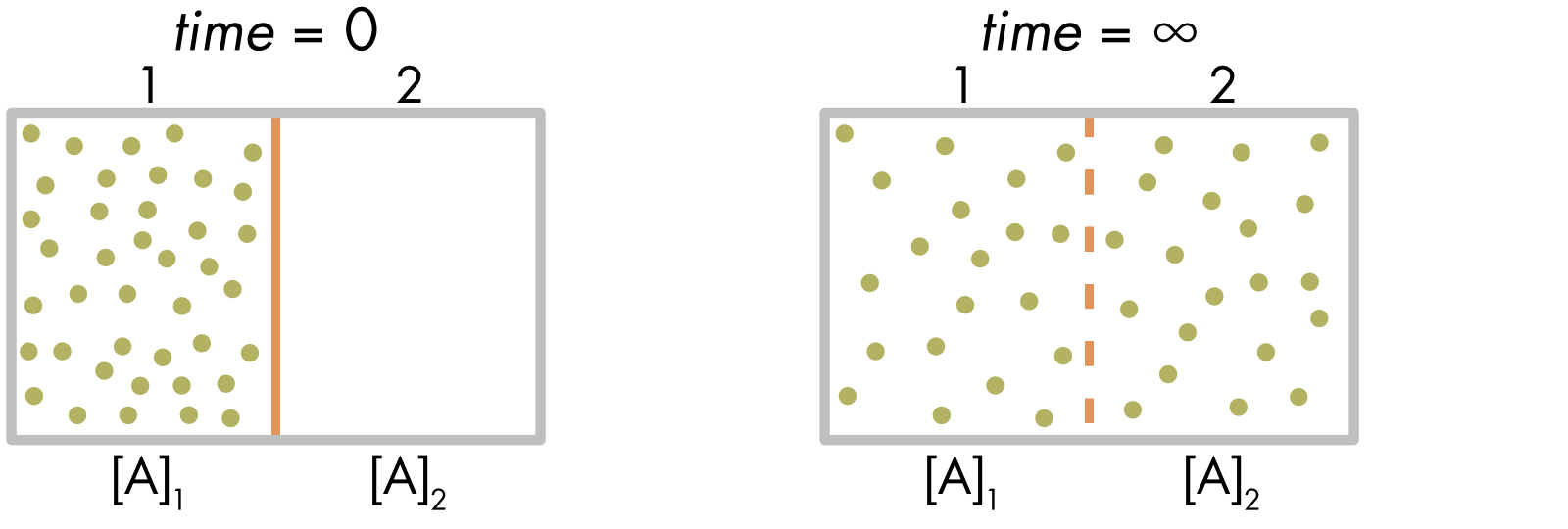
Figure 1 Distribution of solute A between two compartments separated by a membrane. Initially the solute is restricted to one compartment. At time = 0, the membrane separating the two compartments becomes permeable to the solute and solute molecules diffuse into the second compartment until, at equilibrium (time = ∞), there is an equal distribution of the solute between the two compartments.
There are two things to explain. First, why is there an equal number of solute molecules on both sides of the membrane at equilibrium. It is intuitively obvious that this will be the final outcome, but what is the thermodynamic explanation for this result?
Second, at equilibrium, there has been an important change in the system, it has lost the ability to perform work. Initially there was a gradient of solute molecules and the potential energy of this gradient could have been coupled via a membrane transporter to perform work, such as moving a different solute up a concentration gradient from compartment 2 into compartment 1. This capacity to perform work, the potential energy, has been lost at equilibrium. The kinetic energy of the system is unchanged, the water and solute molecules are still in constant movement, and the temperature remains unchanged. The loss of potential energy is accompanied by an increase in entropy — the system is more disordered at equilibrium. We need a way to link the change in the distribution of the solute molecules, the change in the chemical potential energy, with a measure of the change in entropy.
Multiplicity
The thermodynamic explanation for the equal distribution of solute molecules between the two compartments at equilibrium (Figure 1) is statistical. In short, when there are a large number of solute molecules it is vastly more likely that there will be an even, or very close to even, distribution of solute molecules between the two compartments than any other possible distribution.
For the example shown in Figure 1, it can be assumed there are only two possible outcomes for each solute molecule — either it is in compartment 1, or in compartment 2. The distribution of solute molecules between two equal sized compartments can be described mathematically using the binomial equation,
\[W\left( M,N \right) = \frac{M!}{N!\left( M - N \right)!}\]
where, \(W\left( M,N \right)\) is the multiplicity for outcome \((N)\), \((N)\) is the number of solute molecules in a given compartment, and \((M)\) is the total number of solute molecules.
Multiplicity (\(W\left( M,N \right)\)) is the sum of all the ways a particular outcome can occur. Imagine there are only 4 solute molecules in the system. The multiplicity for an equal distribution between the two compartments, can be calculated by setting the number \((N)\) of solute molecules in compartment 1 equal to 2,
\[W\left( 4,2 \right) = \frac{4!}{2!\left( 4 - 2 \right)!} = \frac{24}{2 \times 2} = 6\]
There are six different ways that the four different solute molecules can be distributed between the two compartments to give an equal distribution of molecules between the two compartments (Figure 2). In contrast, there is only one way to order the solute molecules when they are all in compartment 1. Each one of these arrangements is equally likely, since they reflect the random movement of individual solute molecules. As a consequence, it is six times more likely that the molecules will be evenly distributed than all clustered in compartment 1.
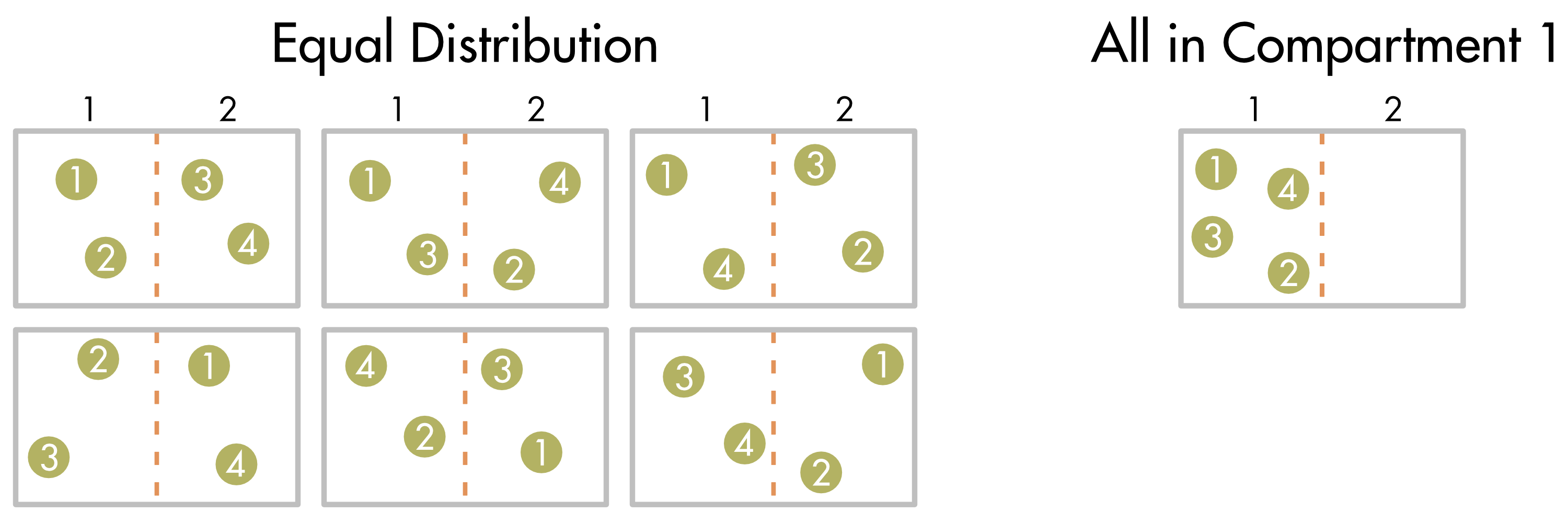
Figure 2 Different ways that four solute molecules can be distributed between two compartments when there is an equal distribution between the compartments (left) or a clustered distribution (right).
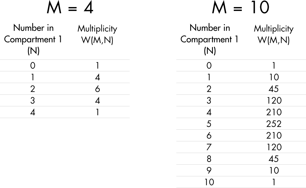
The multiplicity values for all possible ways to order 4 solute molecules are shown in Table 1. As expected, the most common outcome (the outcome with the highest multiplicity) occurs when the two compartments have equal numbers of molecules (in this case when N = 2). There is a total of 16 different ways to arrange these 4 solute molecules. Each one of these different configurations is known as a microstate.
Table 1 Multiplicity for the distribution of four and ten solute molecules in a two-compartment chamber.
The total multiplicity \((W)\), the sum of every possible outcome, is given by,
\[W = 2^{M}\]
For M = 4, W = 16 and there is a 1 in 16 chance that all the solute molecules will be found in compartment 1. This is a low but not insignificant chance. If there are 10 solute molecules (M = 10), then W = 1024 and the probability of all molecules being in compartment 1 falls to 1 in 1,024, a much lower likelihood.
The value for the total multiplicity \((W)\) quickly approaches extraordinarily large numbers as the number of solute molecules increases. For M = 100, W = 1.3 \(\times\)1030, for M = 1,000, W = 1.1 \(\times\)10301, and for M = 10,000, W = 2.0 \(\times\)103010. It quickly becomes vanishingly unlikely that all the solute molecules will cluster in one compartment.
A second important change as the number of solute molecules \((M)\) increases is that the distribution of likely outcomes becomes narrower (Figure 3). For large \((M)\), most outcomes (microstates) other than those very close to an equal distribution of solutes between the two compartments are extremely unlikely.
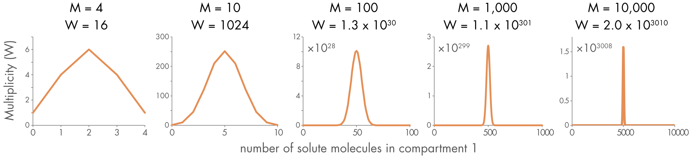
Figure 3 Distribution of multiplicity for different numbers of solute molecules (M) in a chamber with two equal sized compartments.
Even 10,000 solute molecules is a small number compared to the number of solute molecules in a cell. For a 50 µm diameter cell there are approximately 5 × 10¹² potassium ions in the cell. Although a purely statistical argument, the probability that all the potassium ions in a cell might spontaneously cluster in one half of the cell is effectively zero (approximately 1 in \(10^{10^{12}}\)).
For solutes in the cell present in micromolar or higher quantities it is reasonable to conclude that they will always be evenly distributed at equilibrium. For much smaller volumes, very dilute solutes, or systems that are not at equilibrium inhomogeneous distributions of solutes can be important physiologically. Nonetheless, for most purposes we can assume homogeneity.
Entropy
The relationship between multiplicity and entropy is given by the Boltzmann equation,
\[S = \text{k}\,\ln W\]
where, S is entropy, W is the multiplicity of the microstates for a given configuration, k is the Boltzmann constant, and ln is the natural logarithm (ln = loge). Units are joules per kelvin (J\(\cdot\)K-1). This is known as the statistical definition of entropy, there are other ways to define entropy.
In the model described above, the system tends to evolve towards the maximum multiplicity, because this is the highest probability state. Entropy, which is a logarithmic transformation of multiplicity, has a maximum at the same point in the distribution as the maximum multiplicity (Figure 4). For this system, the statement that entropy tends to increase, the Second Law of Thermodynamics, is equivalent to saying that the system will tend towards the most probable state, the state with the highest multiplicity.
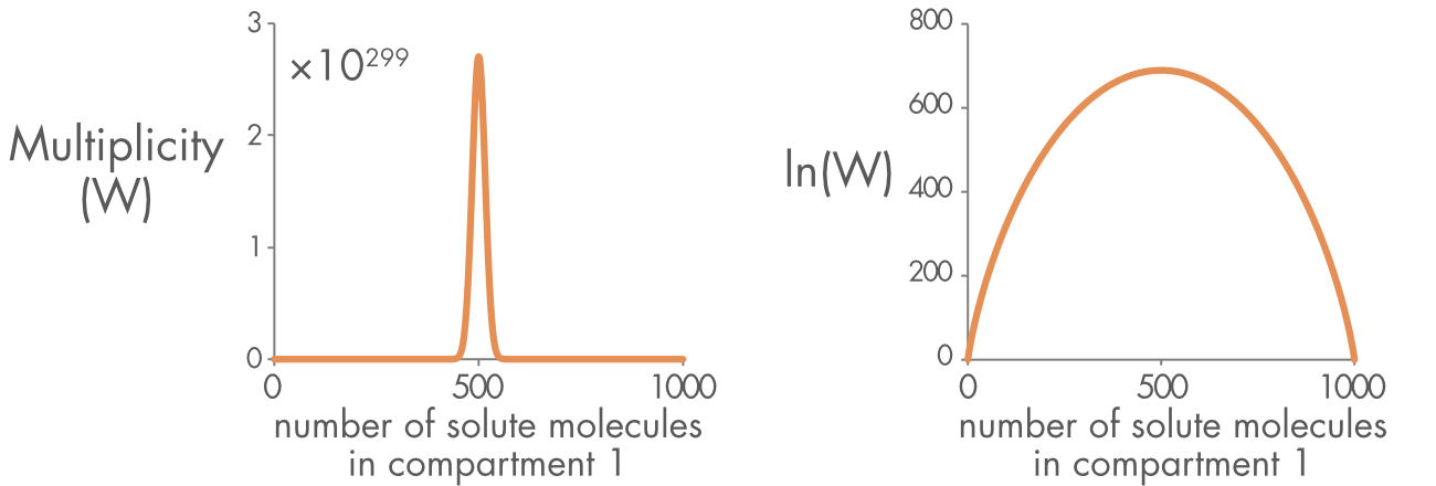
Figure 4 (right panel) Distribution of multiplicity for 1,000 solute molecules in a chamber with two equal sized compartments. (left panel) The natural log (ln) of the multiplicity (W), which is proportional to the entropy (S).
The Boltzmann constant k describes entropy in units of entropy per particle. For biological solutions it is usually more convenient to express entropy per mole of particles,
\[S = \text{R}\,\ln W\]
where R = NAk is the gas constant, and NA is the Avogadro constant, the number of molecules per mole.
Physical Constants
The following physical constants will be used in subsequent sections:
| Gas constant | R | 8.31447 | J\(\cdot\)K–1\(\cdot\)mol–1 |
| Boltzmann constant | k = R/NA | 1.3807 × 10⁻²³ | J\(\cdot\)K–1 |
| Avogadro constant | NA | 6.022 × 10²³ | mol–1 |
| Faraday constant | F | 96,485 | C\(\cdot\)mol−1 |
Gibbs Free Energy
A system held at a constant temperature and pressure, which is generally the case for biological systems, will tend toward its state of minimum Gibbs free energy \((G)\). The change in Gibbs free energy is defined as,
\[\Delta G = \Delta H - T\Delta S\]
where, \(\Delta G\) is the change in Gibbs free energy, \(\Delta H\) is the change in enthalpy, a measure of heat given off (or taken up) by a given process, \(T\) is the temperature and \(\Delta S\) is the change in entropy.
Enthalpy is defined as
\[H = U + pV\]
where U is the sum of the system's internal energy, p is pressure, and V is the volume of the system.
A reaction or process will only go forward spontaneously if the change in Gibbs free energy is negative, i.e. ΔG < 0. For the system described in Figure 1, the change in free energy is given by,
\[\Delta G = {G_{\infty} - G}_{0}\]
\[\Delta G = {(H_{\infty} - TS_{\infty}) - (H}_{0} - TS_{0})\]
There is no change in enthalpy (\(H_{\infty} = H_{0})\) so,
\[\Delta G = - T(S_{\infty} - S_{0})\]
In this example the change in Gibbs free energy is negative solely due to the increase in entropy \((S_{\infty} > S_{0})\).
Three Types of Potential Energy
The transport of ions involves three types of potential energy:
- the potential energy associated with the non-equilibrium distribution of solutes
- the potential energy associated with non-equilibrium chemical reactions, in particular the hydrolysis of ATP, which provides the energy for the generation of ion gradients
- the potential energy associated with the movement of charge in an electric field
These three forms of potential energy can be converted from one form to another. Thermodynamics provides a means of bookkeeping the energy budget for a given process. For this purpose, we require equations that describe each of the three types of potential energy in the same currency (units), which will be joule per mole (J⋅mol-1).
Chemical Potential of Solutes
The chemical potential \((µ)\) of a solute is defined as the Gibbs free energy per mole of solute,
\[\mu = \frac{G}{N}\]
where, G is the Gibbs free energy of the solute, and N is the number of moles of solute. The units for the chemical potential are J⋅mol-1.
The chemical potential is proportional to the logarithm of the solute concentration.
\[\mu = \mu{^\circ} + \text{R}\text{T\ ln}\left\lbrack C \right\rbrack\]
where, \(\mu{^\circ}\) is the standard chemical potential for the solute (measured at 1M concentration), and C is the concentration of the solute.
As might reasonably be expected, the chemical potential for a solute increases as the solute concentration increases.
Chemical Potential for ATP Hydrolysis
To understand the movement of solutes across the membrane by pumps we also need a measure of the chemical potential for ATP hydrolysis. For chemical reactions, such as the hydrolysis of ATP, the change in Gibbs free energy usually depends on both changes in enthalpy and entropy. At constant pressure, the enthalpy of the products and reactants of the reaction equals their total bond energy, and these are rarely equal. If the bond energy of the products is lower (ΔH < 0) the reaction gives off heat and if the bond energy of the products is higher (ΔH > 0) the system absorbs heat.
For chemical reactions the system is not driven solely by an increase in entropy, as was seen above for the diffusion of solutes. There can be a decrease in local entropy if the change in enthalpy is negative and sufficiently large to offset the decrease in entropy.
The key concept to grasp is that the distance a given reaction is from equilibrium determines the chemical potential for that reaction and how much useful work it can potentially perform.
The ATP hydrolysis reaction can be written as,
\[\text{ATP} + \text{H}_{\text{2}}\text{O} \rightleftharpoons \text{ADP} + \text{P}_{\text{i}}\]
At equilibrium, in a test tube, the ATP:ADP ratio is approximately 10-7. The forward reaction goes almost to completion. At equilibrium the chemical potential for ATP hydrolysis is zero. As the distance from equilibrium increases the chemical potential for ATP hydrolysis increases (Table 1).
Table 1 Chemical potential for the hydrolysis of ATP.
| ATP/ADP | Δµ (kJ⋅mol-1) | Condition |
|---|---|---|
| 0.0000001 | 0 | equilibrium |
| 0.00001 | -12 | |
| 0.001 | -24 | |
| 1 | -42 | |
| 10 | -48 | |
| 100 | -53 | |
| 1000 | -59 |
In the cytoplasm of a healthy cell the ATP:ADP ratio is maintained in the range of 10:1 to 1,000:1. In healthy cells, estimates of the chemical potential for ATP hydrolysis are typically greater than -50 kJ⋅mol-1. The mitochondria work furiously producing ATP to maintain this reaction very far from equilibrium in order to create the large chemical potential difference required to drive the processes coupled to this reaction.
Maintenance of this ATP:ADP gradient is essential to maintain the life of the cell. During a stroke there is a disruption of the flow of glucose and oxygen to neurons in the brain. Oxidation of glucose is essential for the generation of the proton gradient in the mitochondria and the production of ATP. As shown in Table 1, as the ATP:ADP gradient declines the free energy for hydrolysis of ATP also declines. If this decline is not quickly reversed the chemical potential for ATP hydrolysis will fall below the level necessary to drive many of the reactions coupled to ATP hydrolysis. Resulting failures include dissipation of the sodium ion gradient and a rise in the internal calcium ion concentration, both of which will contribute to the death of neurons.
Electric Potential Difference
The electric potential is given by,
\[V = \frac{U}{q}\]
where U is the electric potential energy and q is the charge.
The electric potential difference between two points (A and B) is given by,
\[\Delta V = \frac{U_{B} - U_{A}}{q}\]
The electric potential energy difference \({(U}_{B} - U_{A})\) has the units of joules and the electric potential difference \((\Delta V)\) has units of joules per coulomb or volts (V). The difference between these two quantities is analogous to the relationship between Gibbs free energy \((G)\) and the chemical potential (µ) of a solute, except that the chemical potential is expressed in joule per mole (J⋅mol-1). The electric potential can be converted to J⋅mol-1 using the Faraday constant (F).