Signal Processing
Processing of recorded electrical signals is the initial step before analyzing electrophysiological data. Key steps include filtering and analog-to-digital conversion. To understand these manipulations, it is necessary to understand a little about how signals are analyzed.
Signal Analysis
Figure 1 illustrates a remarkable phenomenon. A square wave can be constructed simply by adding together sine waves of decreasing amplitude. As an increasing number of sine waves are added together the signal becomes a progressively good approximation of a square wave.
Figure 1 Sine waves can be added together to create a square wave. The sum of sine waves is shown in red, and the last sine wave (harmonic) added is shown in orange. Increase the number of sine waves (harmonics) that are added into the signal using the button on the right. In principle it is necessary to add an infinite number of sine waves to produce a perfect square wave, but far fewer are required to get a reasonable approximation due to the finite sampling frequency used in this simulation.
To create a square wave the sine waves must be added in a specific way – an infinite sum of odd harmonics of decreasing magnitude.
\[x\left( t \right) = \frac{4}{\pi}\sum_{k = 1}^{\infty}\frac{\sin\left( \left( 2k - 1 \right)2\pi ft \right)}{2k - 1}\]
\[x\left( t \right) = \frac{4}{\pi}\left( \sin\left( 2\pi ft \right) + \frac{1}{3}\sin\left( 3 \cdot 2\pi ft \right) + \frac{1}{5}\sin\left( 5 \cdot 2\pi ft \right) + \cdots \right)\]
where \(f\) is the fundamental frequency.
The square wave example illustrates a general principle, any repetitive signal can be broken down into sine waves of different frequencies (Figure 2).
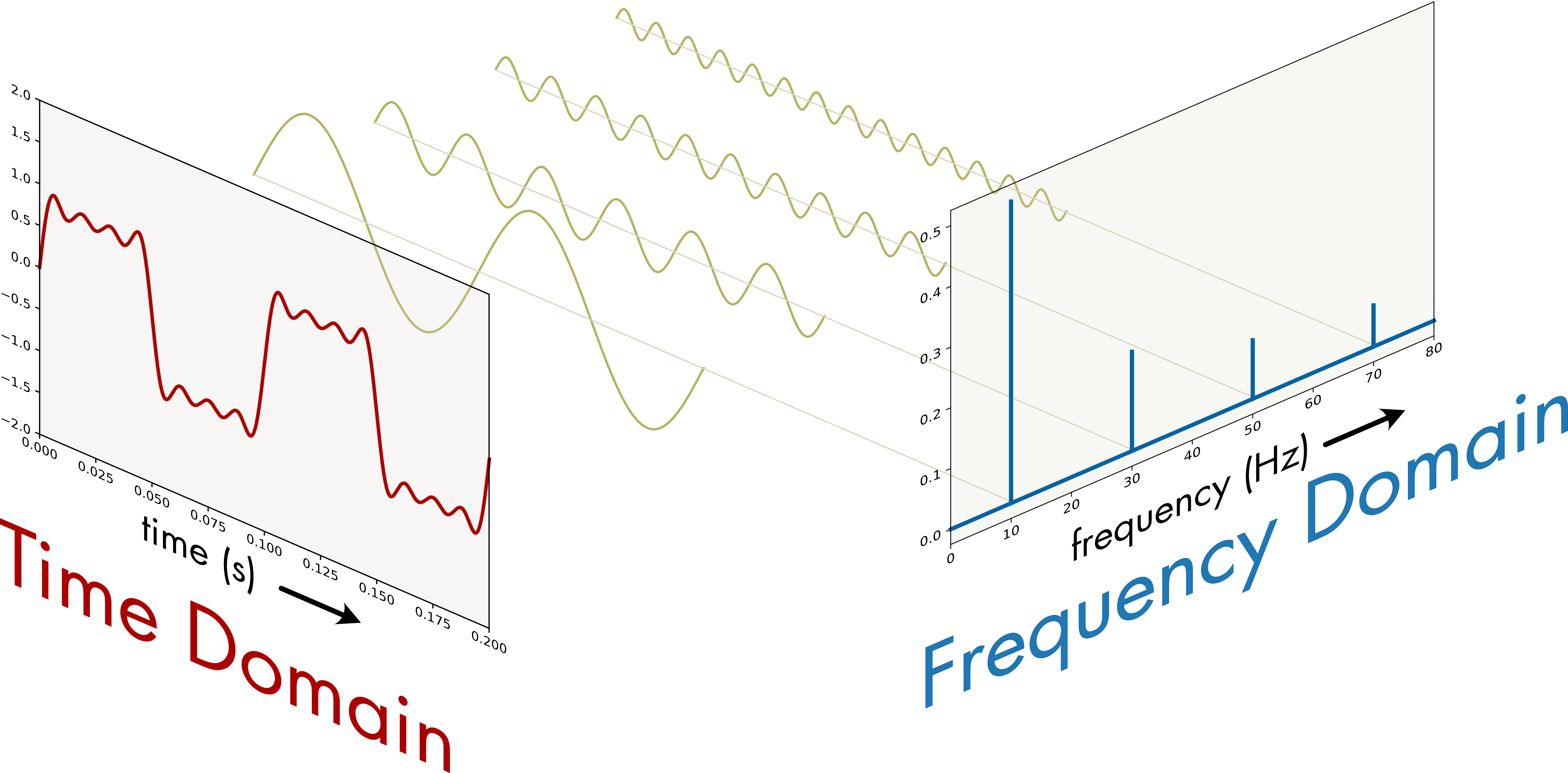
Figure 2 In the time domain a signal comprised of the first four harmonics of a square wave is shown. The signal is then broken down into its constituent sine waves. In the frequency domain the frequency (x-axis) and amplitude (y-axis) of each component is shown.
A signal can be analyzed in both the time and the frequency domains. It can be converted from the time domain to the frequency domain without loss of information using a Fourier transform, which converts a time function into a sum of sine waves with different frequencies, amplitudes, and phase shifts. Time domain signals are converted to the frequency domain because it is often easier to analyze and manipulate signals in the frequency domain.
Continuous-Time and Discrete-Time Signals
Electrophysiological signals are continuous-time functions, known as an analog signal. Analog signals cannot be stored directly in a computer. To store and analyze these signals in a computer the signal must be converted to a discrete-time function—a finite sequence of numbers. The analog signal is sampled at discrete intervals, known as the sampling interval, to create the digitized signal (Figure 3). This process is known as analog-to-digital conversion and the instrument that performs this operation is an Analog-to-Digital Converter (ADC).
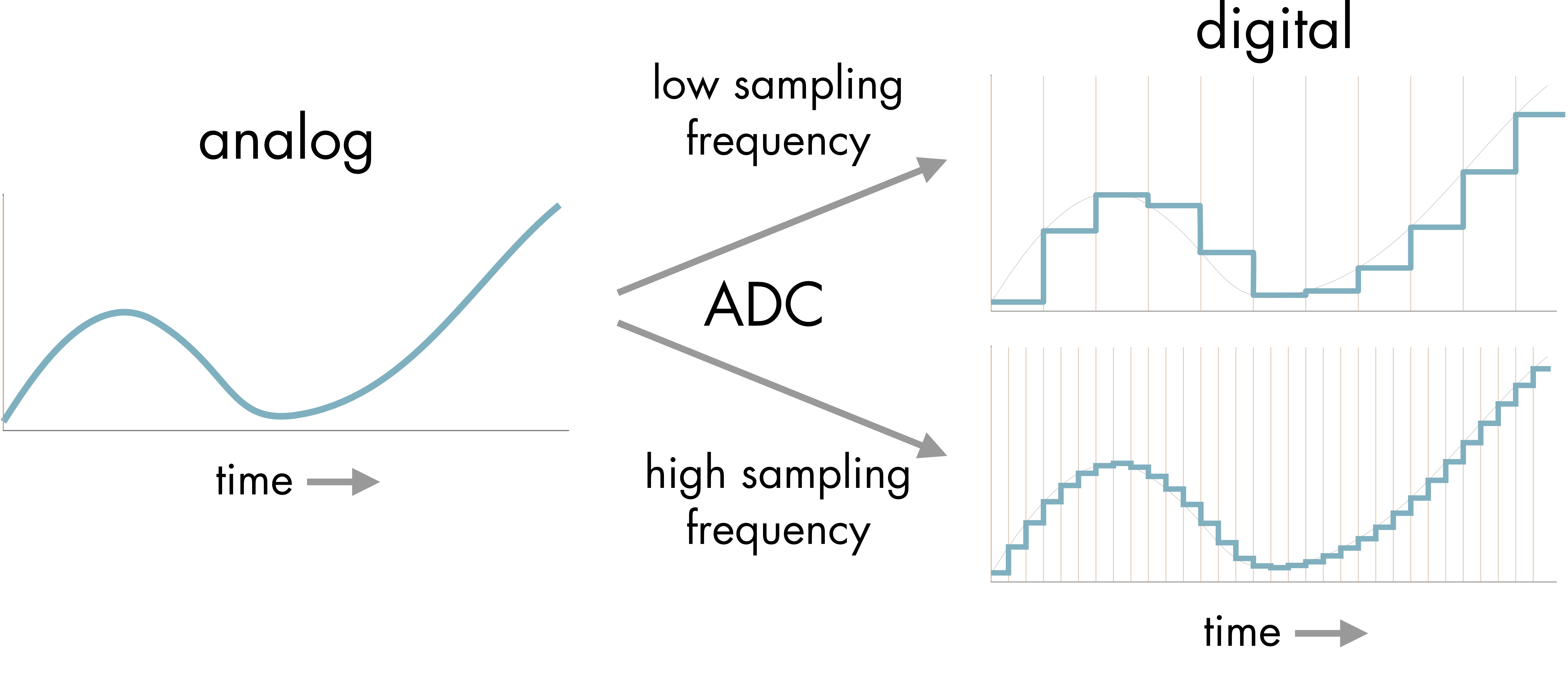
Figure 3 Analog-to-digital conversion. The analog signal is converted to a digital signal using an Analog-to-Digital Converter (ADC) with either a low or high sampling rate. The resulting digitized signal is a time series of discrete values. The sampling interval is represented by the vertical lines.
The quality of the conversion depends on the sampling rate and bit depth. It is intuitively obvious that a higher sampling rate will give a better representation of the signal (Figure 3). Bit depth refers to the length of the number used to represent each sample value. An 8-bit number use 8 binary digits to represent the number, a 12-bit number uses 12 binary digits, and so on. A larger bit depth means that more different voltage levels can be represented in the digital signal.
| Number of Bits | Number of Levels |
|---|---|
| 8 | 256 |
| 12 | 4096 |
| 16 | 65536 |
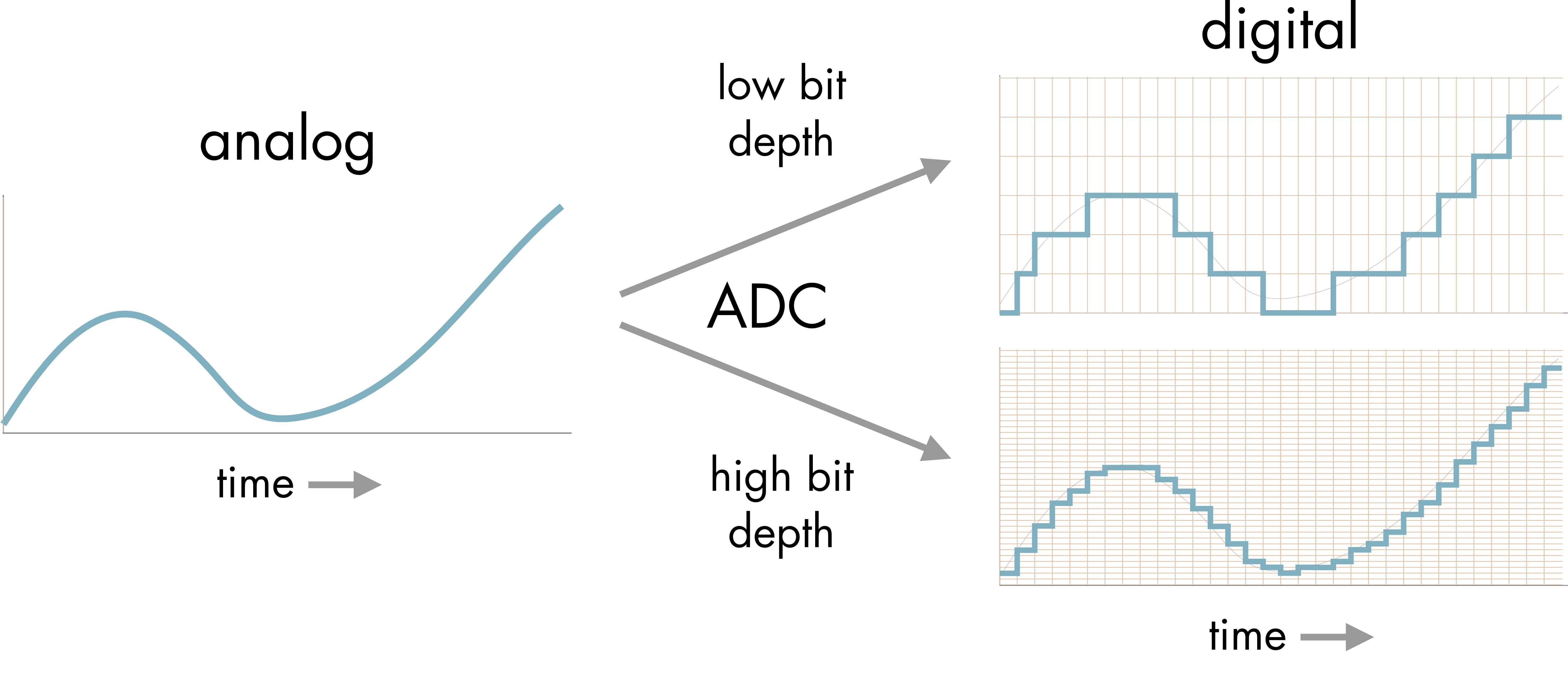
Figure 4 Analog-to-digital conversion. The analog signal is converted to a digital signal using either a low or high bit depth. The number of different levels used to represent the signal are shown by the horizontal lines.
The greater the bit depth of the conversion the more accurate the representation of the signal at each time point (Figure 4). If care is taken, to pick the correct sampling frequency and bit depth, little information of importance will be lost in the analog-to-digital conversion.
Nyquist Frequency
The maximum frequency analog signal that can be represented in a discrete signal is known as the Nyquist frequency. It is half of the sampling frequency,
\[f_{N} = f_{s}/2\]
where \(f_{N}\) is the Nyquist frequency and \(f_{s}\) is the sampling frequency.
This is an important value because if you attempt to sample a signal using a sampling frequency lower than the Nyquist frequency an artifact known as aliasing occurs (Figure 5).
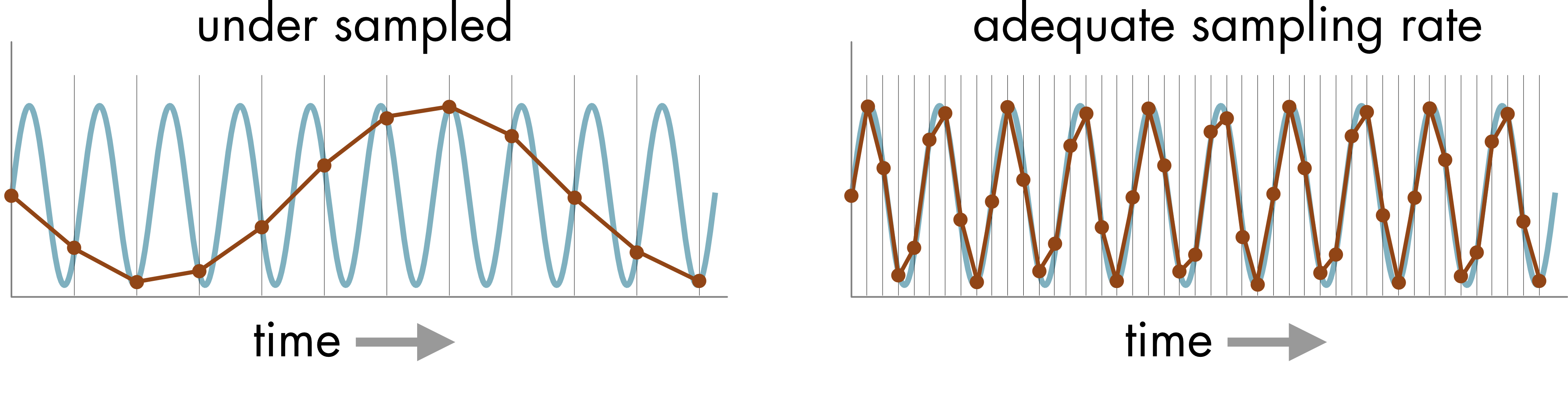
Figure 5 If the sampling rate of the analog-to-digital conversion is too slow relative to the frequency of the signal, aliasing will occur. In the left-hand panel the original signal (blue) was a high frequency sine wave. The sampled signal (crimson) falsely represents this signal as a much lower frequency signal. In the right-hand panel, an adequate sampling rate was used to represent the signal. The sampling interval is represented by the vertical lines.
A rule of thumb is to sample at or above the Nyquist frequency i.e., twice the frequency of the highest frequency signal that you wish to capture, since this avoids distortion of the signal of interest. If there are higher frequency components in the signal, such as noise, these components will be aliased and appear as lower frequency noise in the signal. Typically, it is necessary to use a low-pass analog filter to reduce or eliminate these higher frequencies before sampling (see below in 'Signal and Noise' and 'Filtering').
Discrete Fourier transform
The Fourier transform is used to decompose continuous time functions into an infinite sum of sines and cosines of different frequencies. The Discrete Fourier Transform (DFT) performs a similar decomposition of discrete (digitized) signals.
\[X_{k} = \sum_{n = 0}^{N - 1}x_{n} \cdot \left\lbrack \cos\left( \frac{2\pi}{N}k_{n} \right) - i \cdot \sin\left( \frac{2\pi}{N}k_{n} \right) \right\rbrack\]
where \(X_{k}\) is the discrete Fourier transform, \(N\) is the number of samples, \(n\) is the current sample, \(k\) is the current frequency, and \(x_{n}\) is the sine value at sample \(n\). The discrete Fourier transform has a real and imaginary component and includes both amplitude and phase information.
The algorithm most commonly used to calculate the discrete Fourier transform is known as the Fast Fourier Transform (FFT). As the name implies the FFT can be computed relatively quickly, and it can be used to perform frequency domain analysis in real time for some applications.
The FFT of four different waveforms is shown in Figure 6. The sine wave is represented as a single line in the frequency domain located at the fundamental frequency of the sine wave. When two or four sine waves are present in the signal additional frequency peaks are seen in the frequency domain. The square wave is represented as an infinite series of lines at the odd harmonics of the fundamental frequency in the frequency domain. The amplitude at each harmonic declines with increasing frequency.
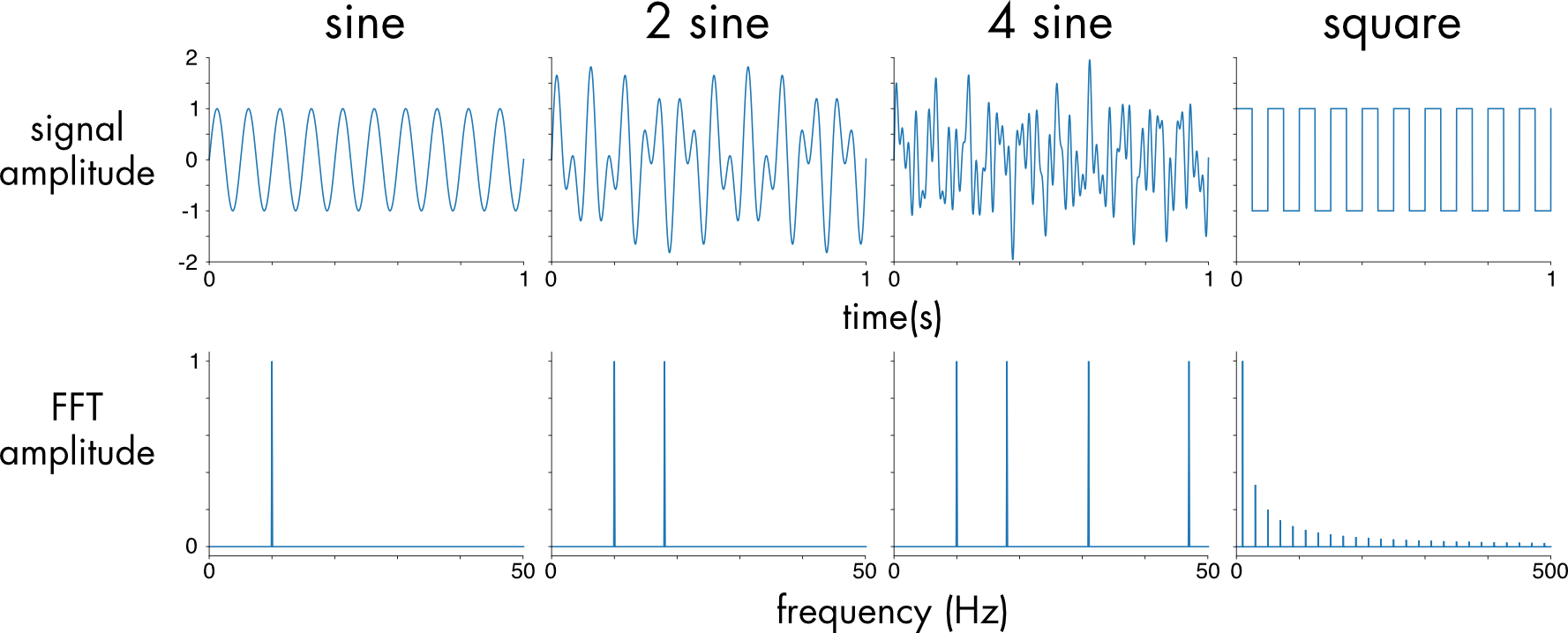
Figure 6 Four different waveforms shown in both the time domain (upper panels) and frequency domain (lower panels). From left to right, a single sine wave (10 Hz), sum of two sine waves (10 + 18 Hz), sum of four sine waves (10 + 18 + 31 + 47 Hz), and a square wave.
In the frequency domain a critical difference between a sine wave and a square wave can be seen. A sine wave is represented by a single frequency component in the frequency domain. In contrast the square wave is very complex, with a literally infinite number of high frequency components. The sharp edges of the square wave in the time domain create these high frequency components. Any very rapid transition in the time domain will be represented by high frequency components in the frequency domain. Because of this difference, sine and square wave signals will be affected very differently by signal processing steps such as filtering and analog-to-digital conversion.
Power Spectrum
The power spectrum density (PSD) is the most commonly used tool in signal analysis. It is typically estimated using Welch’s method. It provides a physical interpretation of the power amplitude rather than just the absolute magnitude given by the discrete Fourier transform and it handles complex noisy signals better than the FFT algorithm because of the averaging inherent to the method. The PSD does not preserve phase information, unlike the FFT. The power spectrum plots the fraction of a signal's power found at each different frequency as a function of frequency.
The power spectrum density is most useful for analyzing noisy signals, which is most signals encountered in biology. There are different types of noise. White noise is a perfectly random signal. The power is distributed equally across the entire frequency spectrum (Figure 7). Pink noise, or 1/f noise, is a kind of noise often encountered in biological systems. The power spectrum declines with increasing frequency, indicating a preponderance of low frequency power in the signal.
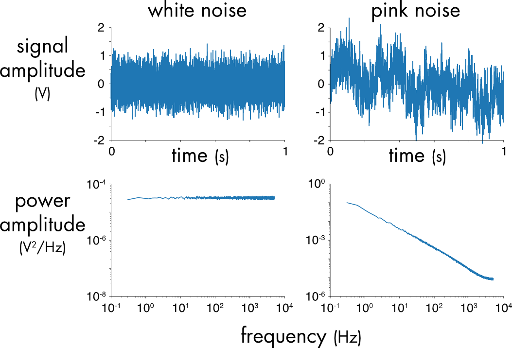
Figure 7 Power spectrum (bottom panels) of white and pink noise (top panels).
The power and frequency values of the PSD analysis are typically plotted on a log-log plot (Figure 7). Log-log plots like these are common in signal analysis because they allow examination of a very broad range of frequencies and amplitudes on the same graph.
Signal and Noise
An electrical signal can be thought of as having two parts, the signal, the part of interest, and the noise, the extraneous part of the signal that carries no useful information (Figure 8).
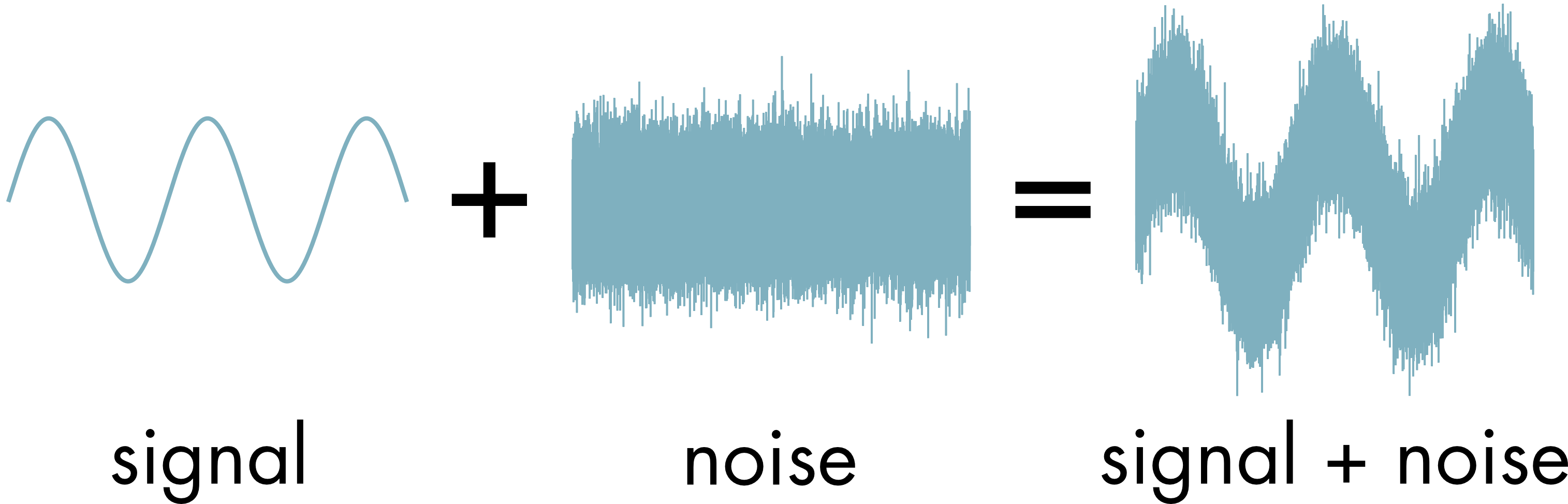
Figure 8 A signal, in this case is a sine wave, and white noise.
The signal to noise ratio (SNR) is often used to describe the relative contribution of both elements. A high signal to noise ratio is obviously preferable although not always achievable.
\[\text{SNR}\ = \ \frac{P_{s\text{ignal}}}{P_{\text{noise}}}\]
where, \(P_{s\text{ignal}}\) is the average power of the signal and \(P_{\text{noise}}\) is the average power of the noise.
Filtering
Filters can be either analog, used on a signal before digitization, or digital, used on a signal after digitization. Functionally there are several broad types of filters, depending on what frequencies they allow to pass (Figure 9).
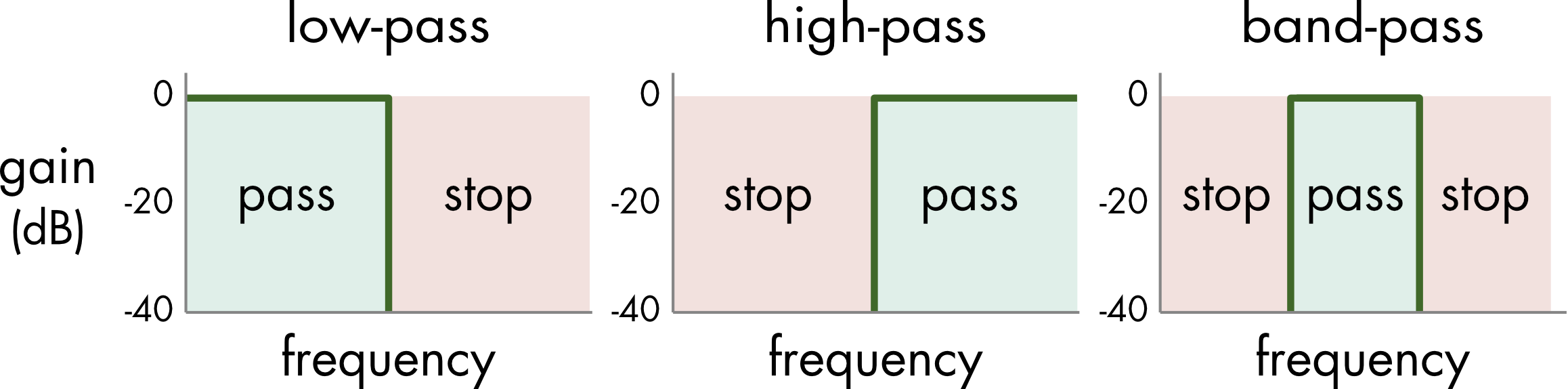
Figure 9 A low-pass filter attenuates high frequencies, a high-pass filter attenuates low frequencies, and a band-pass filter attenuates frequencies outside the pass band. The band of frequencies that are not attenuated by the filter are known as the pass band (green). The stop band (red) is where the signals are blocked or attenuated.
The gain of the filter at each frequency is expressed in decibels (dB),
\[gain = 20\log_{10}\frac{V_{\text{out}}}{V_{\text{in}}}\]
where \(V_{\text{in}}\) is the input voltage, and \(V_{\text{out}}\) is the output voltage. The gain of a filter is typically zero in the pass band, the frequency range where the input voltage is unaffected (Figure 10). The gain is negative in the stop band, the frequency range where the signal is attenuated.
The examples shown in Figure 9 are ideal filters where there is an abrupt transition between the pass and stop bands in the frequency domain. Real-world filters are more complicated. For analog filters it is not possible to create such a perfect transition between the pass and stop bands. The transition is always more gradual. Two key parameters that describe the performance of analog filters are the corner frequency (\(f_{c}\)) and the slope (Figure 10). The corner frequency is the frequency at which the attenuation of the signal is -3 dB. This value is usually adjustable. The slope corresponds to the how quickly the pass band transitions into the stop band and depends on the filter design.
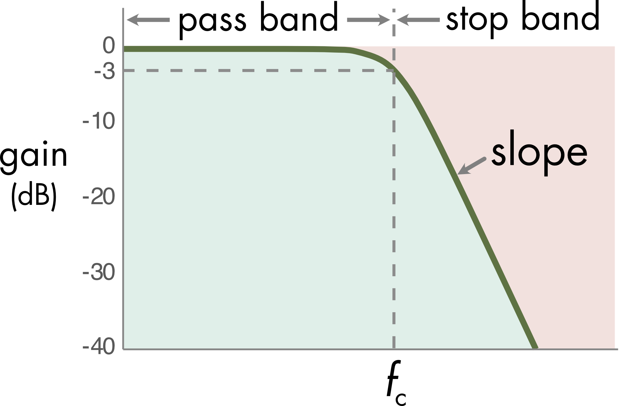
Figure 10 Properties of a low-pass filter. The corner frequency is the frequency at which attenuation of the input signal is -3 dB. The slope describes the performance of the filter after the corner frequency. A steeper slope is closer to an ideal filter.
Filters have several uses in signal conditioning for electrophysiology. Low-pass analog filters are used universally to remove high frequencies before digitization in order to avoid the aliasing artifacts described above. A second use is to reduce the amount of noise contaminating the signal. This step can be performed using either analog or digital filters. There are trade-offs with noise filtering as illustrated in Figure 11.
Figure 11 A 5 Hz sine wave with white noise. Change the corner frequency of the filter by pressing the buttons.
As the corner frequency of the filter is decreased the noise is gradually filtered out but starting around \(f_{c}\) = 100 Hz the signal, a 5 Hz sine wave, also becomes attenuated. The filter has two effects, a desirable reduction of noise and an undesirable distortion of the signal. Since there is usually some overlap in the frequencies of the noise and the signal it is difficult to completely remove the noise without also distorting the signal.
If you look carefully, you can see that the phase of the signal also changes when the filter is set to lower corner frequencies. This phase shifting can be an issue when attempting to correlate timing between events. Zero-phase shift filters can be implemented as digital but not analog filters. In general, the most flexible approach to filtering is to over-sample the data i.e., sample at higher frequencies than necessary using a high corner frequency setting on the anti-aliasing filter. A digital filter can then be applied as needed to reduce noise in subsequent data analysis.
Averaging
For some types of signals, particularly evoked signals, it is possible to average over multiple trials. Because the noise is usually random, averaging reduces the noise without affecting the signal if the signal is close to identical from trial to trial. For random noise the signal to noise ratio will increase in proportion to the square root of the number of trials that are averaged and there is diminishing improvement with increasing numbers of trials. Much of the benefit of averaging can be obtained with a relatively small number of trials.
Although low-pass filtering is effective at removing high frequency noise, as seen above, it is less effective with pink (1/f) noise, which has more power in the low frequency components. Often averaging is the only option to reduce this low frequency noise contamination (Figure 12).
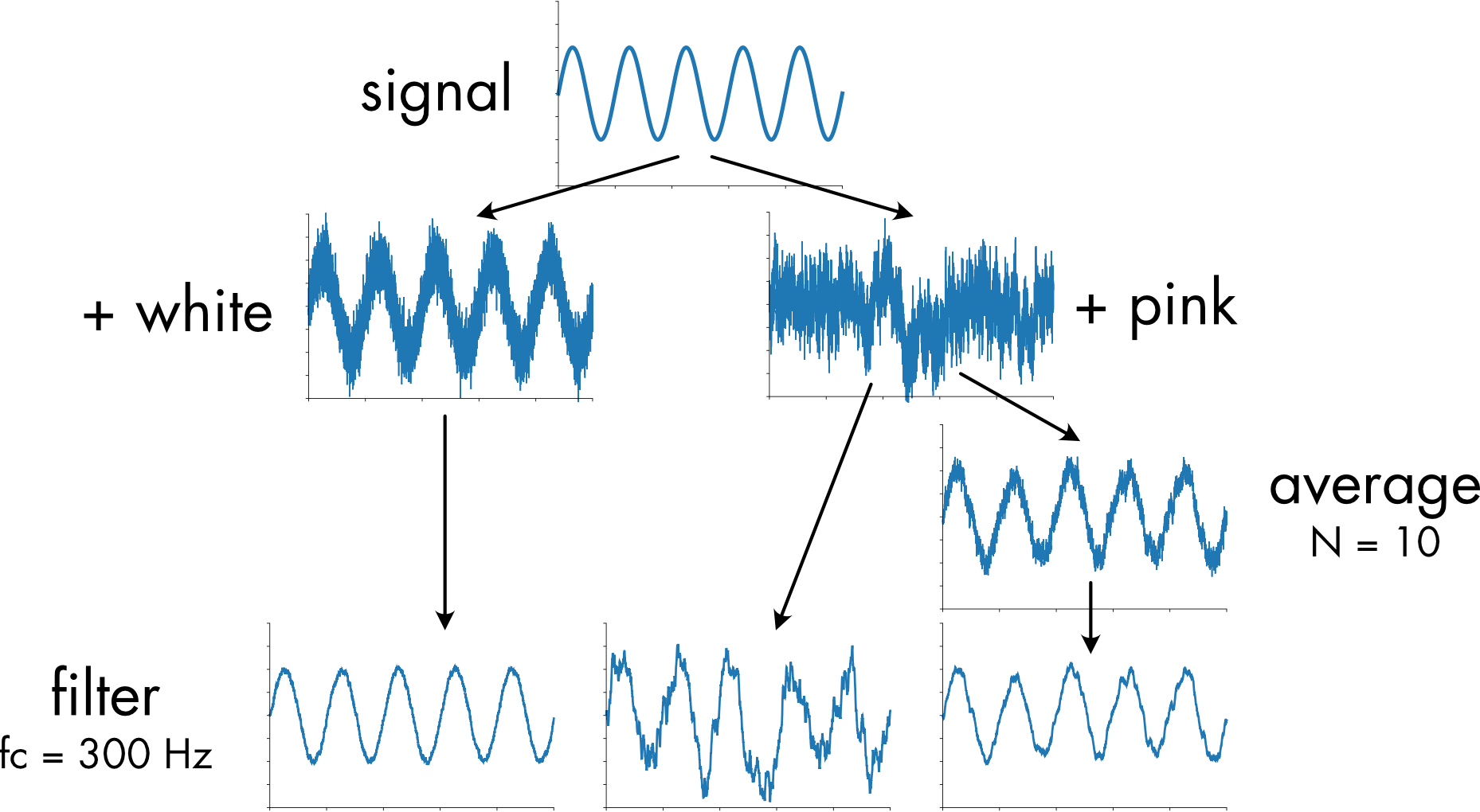
Figure 12 Effects of filtering and averaging on signal plus either white or pink noise. A corner frequency of 300 Hz was used for the filter and ten traces were averaged.
Filtering at 300 Hz removes most of the power in the white noise contaminated signal without significantly distorting the signal. When the signal is contaminated with pink noise it is almost impossible to discern the original sine wave signal due to the presence of low frequency noise components. Filtering by itself cannot remove this low frequency noise. A combination of averaging and filtering is necessary to get a reasonable reproduction of the original signal.